RTLS Toolbox
The RTLS (Real Time Localization System) Toolbox, is a collection of RTLS techniques that can be implemented on TI’s standard Bluetooth Low Energy radios in the CC26xx series. These techniques provide raw data that can be utilized for developing localization algorithms and secure range bounding other Bluetooth Low Energy nodes. The three main techniques included in the RTLS toolbox is RSSI, Angle of Arrival, and TI Time of Flight.
RSSI details the Received Signal Strength Indication of an incoming signal and is commonly leveraged for deriving the distance between a receiver and a transmitter through the process of trilateration in localization algorithms. The Bluetooth Low Energy stack enables developers to receive the RSSI of an incoming Bluetooth packet.
Angle of Arrival (AoA) is a technique for finding the direction that an incoming Bluetooth packet is coming from, creating a basis for triangulation. The device samples an incoming constant tone and as I/Q data. This raw I/Q data represents the amplitude and phase data of a signal and this data can be used to derive the angle the device transmitting the constant tone. TI’s AoA solution on the CC2640R2F is proprietary and only intended for evaluation.
TI Time of Flight is a proprietary technique used for secure range bounding a device by measuring the round trip delay of an RF packet exchange. By taking multiple samples, a result with much better accuracy can be extracted providing developers the data to help trilaterate a device.
Using the raw data provided by the RTLS Toolbox, TI is enabling developers to improve localization algorithms based on Bluetooth technology by delivering more data that can be leveraged for trilateration and triangulation.
The inherent flexibility of the CC2640R2F RF Core is what enables this significant extension of functionality. The main advantages using the CC2640R2F are that customers can start adding RTLS features and security with little extra cost, very little extra energy consumption and no increase in peak power.
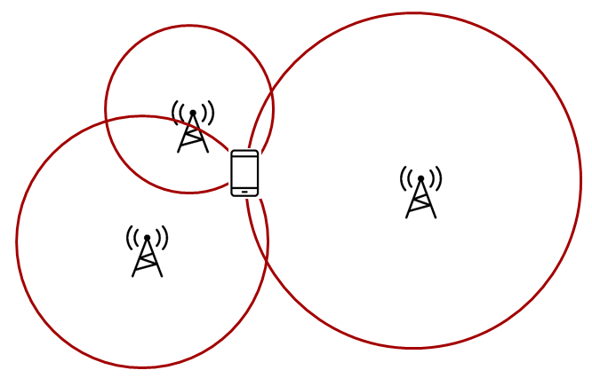
There are two fundamentally different approaches for localization:
| Trilateration | Triangulation |
|
|
Trilateration is where you know the distance between a reference node and a target node. This means that the possible locations seen by one locator constitute a circle, so typically three locators are needed to find a single common intersect point. (Assuming a 2D scenario) Time of Flight gives you the distance from the receiver to the transmitter. |
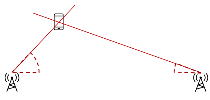
Triangulation is where you know the direction from a reference node to a target node. This means that the possible locations seen by one locator constitute a straight line, so two nodes will be enough to determine a single intersect point. (Assuming a 2D scenario) Angle of Arrival gives you the angle from the receiver to the transmitter. |
Note
Existing examples with no external control interface are discontinued. All RTLS examples now have an external control interface.
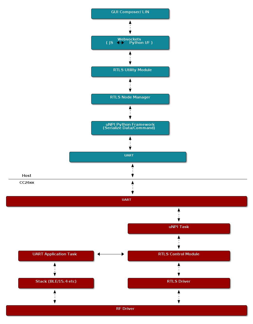
General RTLS Software Architecture
The diagram below shows the RTLS software architecture.
With multiple nodes that collect localization data, it is important to have an architecture that supports control of these nodes. It must be possible to configure and trigger localization and it must be possible to retrieve localization data. We achieve this by reuse of our Network Processor Interface (NPI). It is basically a means to support Remote Procedure Calls (RPC) over a serial interface. Note that the architecture is such that it is possible to replace NPI with your own preferred serial protocol.
In our example we use UART as the serial transport layer. This is because it is readily available on host PC as UART over USB, and our LaunchPads include a UART to USB bridge. Along with the embedded examples we provide PC software to act as host, to control, retrieve and present localization data. This also allows much quicker customer performance characterization, as well as configuration of important parameters, not to mention the ability to develop and test higher level post-processing algorithms.
RTLS Toolbox
The RTLS toolbox is a collection of software that is purposed for the localization use case. A table below summarizes each software component in the toolbox as well as its applications for localization. The software components below will run on the embedded nodes.
| Software Component | Usage |
|---|---|
| BLE-Stack | Advertising, scanning, connection, exchanging RTLS data |
| Connection Monitor | Follows a BLE connection using Micro BLE-Stack |
| Angle of Arrival | Radio patches and driver to read AoA data embedded in BLE packets |
| Time of Flight | Radio patches and driver to send, receive, and observe ToF exchange |
| Unified Network Processor Interface (UNPI) | A serial protocol including packet format and handshaking for power savings |
| RTLS Control Module | Implements the command and event set used to communicate RTLS information between devices. This runs on the embedded devices and translates UNPI frames into the necessary AoA and ToF function calls |
The software components in the following table run on a PC. TI has setup a PC based environment to facilitate in evaluating and prototyping various RTLS algorithms. Once the algorithms are complete, the various PC components above can be migrated to an embedded device.
| Software Component | Usage |
|---|---|
| RTLS Util | Event handling and distrution across nodes. Implements results queues, and setting up worker threads for data handling. |
| RTLS Node Manager | Framework for sending and receiving RTLS commands and events from the embedded devices to PC. Implements higher level logic such as forwarding necessary BLE connection information to the connection monitor node. |
| Websocket Server | Implements the server side of a TCP socket. Intended to bridge serial connections over UNPI from the node manager to TI GUI composer app |
| RTLS Manager GUI Composer App | A simple GUI for aggregating and logging RTLS communication and graphing AoA or ToF data. This is Javascript based and runs in the web browser |
RTLS Utility
The RTISUtil module is a convience layer that is built on top of the node manager that implements event handling and blocking as required by the RTLS network (e.g. seed distribution). Additionally the RTLSUTil module is able to setup worker threads for data processing of results from the device as well as creating queues to store the incoming data.
RTLS Node Manager
The RTLS Node Manager provides the following functionality:
- A bridge between GUI composer and CC2640R2F
- Holds the state of each device and takes care of configuration
- Enables the simplicity of RTLS Control Module and GUI Composer
- Minimizes amount of the transactions between GUI Composer and the rest of the system
Due to the above functionality, the Node Manager can operate on user’s CPU and help with slow bus (LIN/CAN).
RTLS Control Module
The RTLS Control Module is an on-chip module which runs as a RTOS Task and it provides the following functionality:
- Parsing commands coming from Node Manager
- RTLS Driver configuration and operation
- RF and NPI message queue
RTLS Roles and Topology
Each node in an RTLS network utilizes the software components listed above in a
different way to perform a specific task related to localization. These
capabilities map to a role within the RTLS network and ultimately are implemented
by sample applications within the SDK. There are three examples: rtls_master,
rtls_slave, and rtls_passive. The capabilities of these examples are
explained below. All embedded nodes implement UNPI and act as slaves in the UNPI
protocol. Additionally all embedded nodes have the RTLS Control module implemented
for processing RTLS commands from the UNPI interface.
Note
The following subsections aim to describe what localization roles are implemented by the sample applications in the SDK. This is not a comprehensive list of what is possible on each node, but rather an explanation of what the examples will do out of the box. For a list of potential combinations, please see Role Combinations.
Master
The RTLS master runs a full BLE-Stack and acts as a central device. It will scan and connect to the RTLS slave over BLE. Once a connection is established the RTLS Master will do the following:
- Share the connection parameters (access address, master sleep clock accuracy, and CRC init) with the PC.
- Use the BLE link to share ToF and AoA parameters with the peripheral device.
- Implements the ToF master role
- Does not send out AoA packets, but configures the slave to do so.
Slave
The RTLS slave runs a full BLE-Stack and acts as a peripheral device. This is the device that is to be located. The slave device will advertise and enter a connection with the RTLS Master.
- Sends data packets with AoA tone embedded using Constant Tone Extension (CTE)
- Advertises special string to be detected by
rtls_master- Implements ToF slave role
- BLE-Stack peripheral role
- Wireless/battery operated, not connected to PC
Passive
The RTLS passive does not actively participate in the BLE connection between the RTLS master and slave. Instead, it uses the Micro BLE Stack in connection monitoring mode to follow the connection. To do this, the passive device relies on the Master to distribute the connection parameters once a connection is formed. The passive node does the following:
- Implement ToF passive role
- Receives packets with CTE and performs in-phase and quadrature component (IQ) sampling
- Implements the Micro BLE-Stack connection monitoring applciation layer. See Connection Monitor (CM) Application for more information on the connection monitor.
PC/Central Processing Node
The PC node is responsible for controlling the embedded RTLS nodes by sending commands and processing events. In the SDK, this is realized by a combination of a Python layer that implements the UNPI master role and a websocket server that translates UNPI commands to a socket interface that is used by the GUI Composer application running in the browser.
This software is intended to use as a framework for extracting data from the embedded nodes and using it to prototype high level RTLS algorithms on the PC.
Note
In a final product, these algorithms may be implemented on an embedded device or even perhaps the RTLS master node. TI has provided PC software to aid in data plotting and prototyping various algorithms.
The PC implements the following roles in Python:
- UNPI master
- COM port interface
- Implementation of RTLS UNPI subsystem/command set
- Websocket server
The PC implements the following roles in GUI Composer/Javascript:
- Websocket client on localhost
- Graphing and logging data from websocket
- Parsing JSON objects to extract RTLS data
- Issue commands to RTLS nodes via websocket to UNPI conversion
- Enumerate devices
- Distribute connection parameters to passives
Role Combinations
Note
In all of the tables following (BLE, ToF, AoA) features listed as optional are not implemented by the sample applications included in the SDK, but are valid and possible configurations that can be implemented by the user.
For example: rtls_master could be a multi-role device or rtls_passive could
operate as ToF master.
BLE-Stack
The Bluetooth Core Specification Version 5.1 allows for devices to operate in various roles as well as combinations of roles. The table below shows the required and optional features for each example.
| Example Name | Central | Peripheral | Broadcaster | Observer |
|---|---|---|---|---|
| RTLS Master | R | O | O | R |
| RTLS Slave | O | R | R | O |
| RTLS Passive | No | No | O | R* |
Legend:
- R: Required
- O: Optional
- No: Not supported
Note
The R* above denotes that while the connection monitor is capable of scanning
for beacons, it is also required that the connection monitor follow a connection.
The monitoring role is not officially defined by the Bluetooth Spec, but it is
a critical functionality in the rtls_passive.
ToF
ToF roles may be rotated between the RTLS master and RTLS passive. This is a desirable feature because it increases spatial diversity which makes the system more robust against multi-path fading. The following table lists valid configurations for ToF.
| Example Name | ToF Master | ToF Slave | ToF Passive |
|---|---|---|---|
| RTLS Master | R | N/A | O |
| RTLS Slave | N/A | R | N/A |
| RTLS Passive | R | N/A | R |
Legend:
- R: Required
- O: Optional
- No: Not supported
- N/A: Not applicable
AoA
The Bluetooth Core Specification Version 5.1 defines multiple roles for both connected and connection-less AoA. The following configurations are supported by the examples in the SimpleLink CC2640R2 SDK.
| Example Name | Send CTE | Perform IQ Sampling |
|---|---|---|
| RTLS Master | No | No |
| RTLS Slave | R | No |
| RTLS Passive | N/A | R |
Legend:
- R: Required
- O: Optional
- No: Not supported
- N/A: Not applicable
RTLS Driver
The purpose of RTLS Driver is to handle the Direct Call implementation of the RTLS module.
For more detail please take a look at ToF Driver section and AoA Driver section.
Physical Considerations
Before evaluating the RTLS solution, it is important to consider the environment. All radio communication protocols can be susceptible to multi-path fading, and RTLS based systems are not exempt. It is important to control the environment when evaluating or at least be aware of the potential effects of multi-path on the results.
It is recommended to evaluate the RTLS solution in an area that optimizes RF conditions. This includes:
- An open space with no large metal or concrete obstructions (pillars, poles, etc)
- Relatively few interference sources (i.e. Wi-Fi access points, etc)
- Raised platforms for the nodes made out of cardboard ~1 m off the ground.
A desk environment generally has sub-optimal RF conditions and should be avoided.
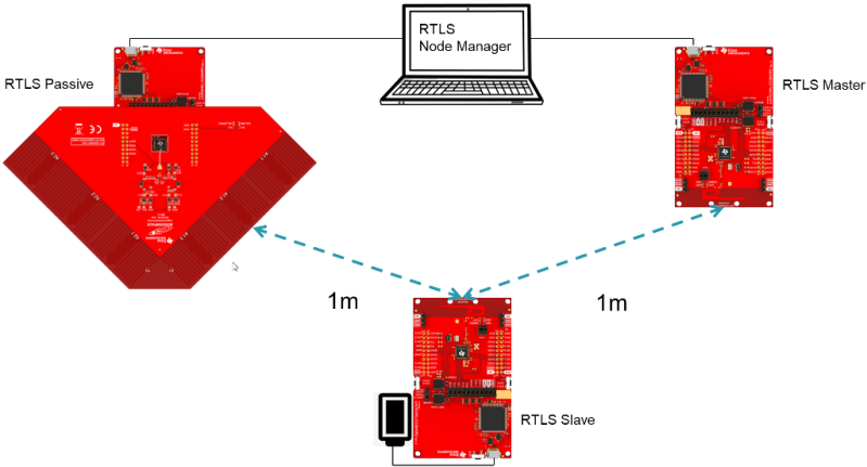
See the image below for a recommended layout of the nodes during evaluation, this is a 2D image where all devices are laying on a flat surface “pointing” as shown in the picture. In this case each node should be placed on a box so that it does not sit directly on the ground.
For angle of arrival application, we have created Bluetooth Angle of Arrival Antenna Design to further explains what users should look for when making their own AoA board.
RSSI Based Localization
RSSI details the Received Signal Strength Indication of an incoming signal and is the most commonly used method of trilateration localization in Bluetooth. TI Bluetooth low energy stack enables developers to receive the RSSI of an incoming Bluetooth packet with can be used to enable RTLS algorithms.
RSSI localization is based on the the Frii’s Transmission Equation. The core concept is that received signal strength is proportional to the distance of the transmitting node. The graphic below describes how RSSI can be used to estimate distance.
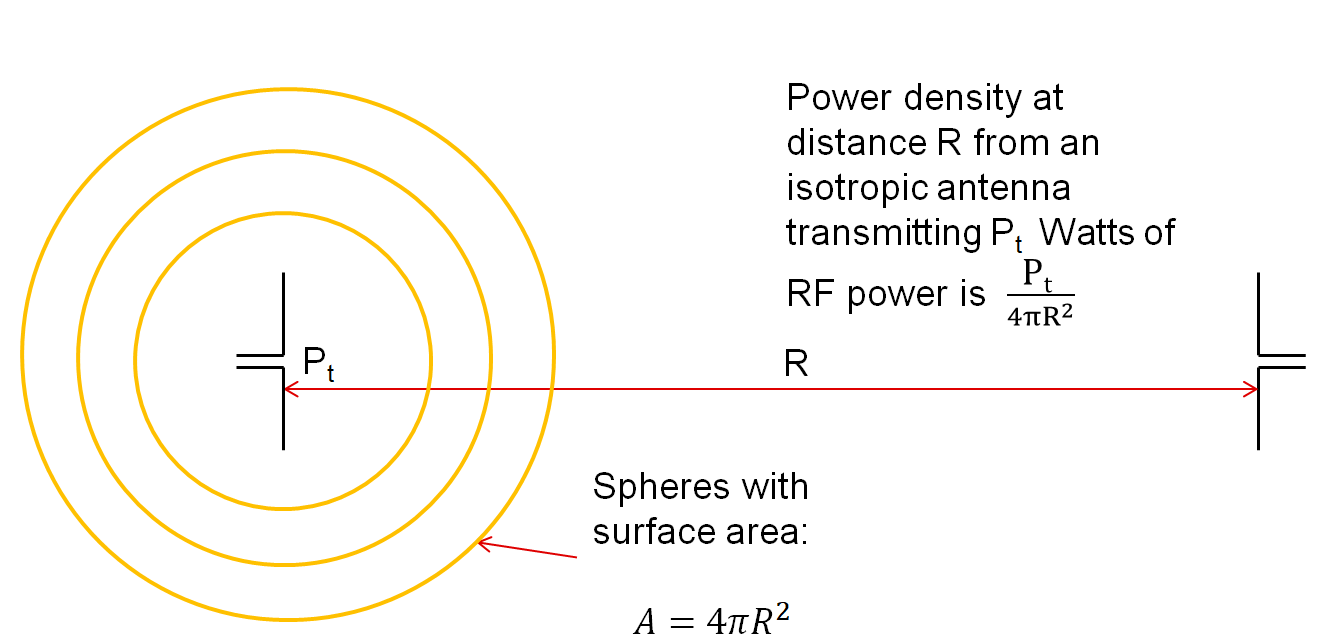
Figure 76. Frii’s Equation Relationship between received power and distance.
While RSSI based localization is the most commonly used method in today’s RTLS systems, it also faces challenges that need to be overcome:
- Accuracy can be influenced by the presence of reflections and obstructions
- No Relay Attack protection
Some of these challenges with RSSI can be overcome through smart system design. TI’s RTLS Toolbox enables developers to monitor the connection between a master and slave and get independent RSSI measurements from the same packet via the Connection Monitor. This approach gives more data and reference points that can be used to help improve the resolution of an RTLS application.
For future RTLS applications, it is recommended to combine RSSI with the other localization techniques such as AoA or ToF to help improve the accuracy and security.
Reading RSSI
The Micro BLE Stack. (foundation of the Connection Monitor (CM) Application) and the full BLE-Stack provide APIs to read RSSI information of the received packet. The following sections will describe how to extract RSSI information from the received packet.
Connection Monitor
The connection monitor will keep an array of connection information
for each connection it is tracking. This includes master and slave RSSI
from the last scan. These fields can be found in the ubCM_ConnInfo_t
structure. The fields are rssiMaster and rssiSlave respectively.
RSSI information is valid after the monitor complete callback is invoked (when the monitoring scan is complete for a connection event).
The rtls_passive sample application shows an example of extracting
slave RSSI in RTLSPassive_monitorCompleteEvt.
BLE(5)-Stack
When using the BLE-Stack, the Gap_RegisterConnEventCb (Generic Access Profile (GAP)) will provide
RSSI from the last connection event. It can be used in the central or peripheral
configuration. The connection event callback is already the synchronization
method used by the RTLSCtrl module for reporting data to the PC/Node
Manager. See Gap_ConnEventRpt_t for information on how to extract
the RSSI from connection event callbacks.
Angle of Arrival
Angle-of-Arrival (AoA) is a technique for finding the direction that an incoming Bluetooth packet is coming from, creating a basis for triangulation.
An array of antennas with well-defined properties is used, and the receiver will switch quickly between the individual antennas while measuring the phase shift resulting from the small differences in path length to the different antenna.
These path length differences will depend on the direction of the incoming RF waves relative to the antennas in the array. In order to facilitate the phase measurement, the packet must contain a section of constant tone (CT) where there are no phase shifts caused by modulation.
Packet Format
In order to get a good estimate of ϕ (phase), all other intentional phase shifts in the signal should be removed.
Bluetooth Core Specification Version 5.1 introduces AoA/AoD which are
covered under Direction Finding Using Bluetooth Low Energy Device section
and it also specifies the following
states can support sending direction finding packets:
- Periodic advertising; also called
Connectionless CTE - Connection; also called
Connection CTE
The theory behind AoA/AoD and Connectionless/Connection CTE(Constant Tone Extension) is the same, therefore, we will only focus on Connection CTE AoA, which is what we currently provide in SimpleLink CC2640R2 SDK
First we will take a look at the payload. By adding a section of consecutive 1’s at the end of connection packet, effectively transmitting a single tone at the carrier frequency + 250kHz.
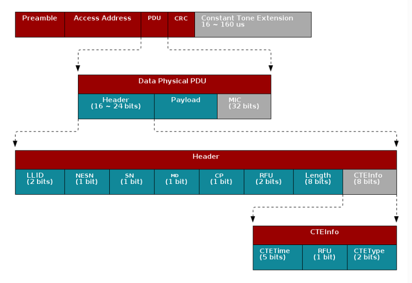
In the header, the CP bit (CTE Present)determines whether header
contains CTEInfo or not.
The CTEType field of CTEInfo further specifies which type of direction finding
packet this is and the CTETime field specifies the duration of the CTE.
Table 20. CTEType value¶ Value Description 0 AoA CTE packet. 1 AoD CTE with 1 µs slots. 2 AoD CTE with 2 µs slots.
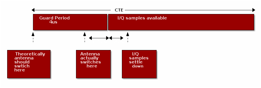
The value of CTETime should be within 2~20 and it’s interpreted as in 8us unit. That means when CTETime is set to 20, there will be CTE at the end of connection packet which lasts 8*20 = 160(us).
This gives the receiver time to synchronize the demodulator first, and then store I and Q samples from the single tone 250kHz section at the end into a buffer and the buffer can then be post-processed by an AoA application
Note
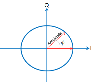
The I/Q Data Sample is the coordinates of your signal as seen down the time axis. In fact, I/Q data is merely a translation of amplitude and phase data from a polar coordinate system to a Cartesian (X,Y) coordinate system and using trigonometry, you can convert the polar coordinate sine wave information into Cartesian I/Q sine wave data.
Integration
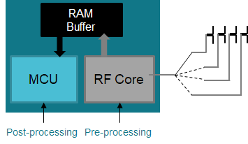
Using a special RF Core patch in receive mode, the I and Q samples from the transmitted carrier frequency + 250kHz tone can be captured, pre-processed, and buffered by the RF Core without any load on the main MCU.
Due to the pre-processing, the application can determine the phase shift without having to remove DC offset or IF first, significantly simplifying the estimation process and leaving the application MCU free to do more on top.
The I/Q sampling rate is configurable and can be up to 4 MHz. Each I/Q pair occupies 32 bit space in radio RAM and the radio RAM can only store up to 2KB(2048 bytes).
Therefore with sampling rate 4MHz, there will be 16 I/Q pairs every 4us, which equals to 16 * 4(one I/Q pair takes up 4 bytes space) = 64 bytes per 4us.
That means even if the CTE is 160us long with 4MHz sampling rate, the radio RAM can only store I/Q data for 128us duration. To ensure that I/Q sample are captured till the end of the tone, we should consider decrease the sampling rate to cover this case. For more information regarding the sampling rate, please see Table 22..
Note
I and Q samples only have 13 bits resolution even though they occupy 16 bits space in radio core RAM. Since they only have 13 bits resolution, the maximum and minimum value you will observe as signed integers are [4095, -4096].
The RF Core can provide event which can be mapped to DMA to trigger the start of GPTimer. The GPTimer is configured as 4us count down mode, once it reaches 4us, then it will generate another DMA transaction to toggle antenna switches.
In slave device, the RF Core patch ensures that the CTE is inserted at the end of the connection event packet without being distorted by the whitening filter.
In passive device, the RF Core patch analyzes the packet and starts capturing samples at the right time while synchronizing antenna switching. The samples are left in the RF Core RAM for analysis by the main MCU
AoA Driver
The AoA driver is responsible for antenna switching and data extraction.
Note
As stated in Integration, in this release only
rtls_passive device can capture I/Q sample and triggers the radio event
for application to do antenna toggling.
Data Collection Flow
Most the code snippet in this section is included in AoA.c.
The radio configuration is in urfi.c.
When radio core detects AoA tone info in the received packet,
it can trigger an radio event called RFC_IN_EV4 and we can route
the event to DMA channel 14 as a start trigger for antenna switching.
GPTimer 0A is configure as periodic down with 4us timeout and the timeout(timer match) event is routed to DMACH9 to trigger antenna toggling.
When there is AoA packet received (AOA.c), DMA will transfer patterns to toggle the antennas on the BOOSTXL-AoA board.
RF core triggers an event 3.25us into the tone.
Therefore to achieve 4us guard time, the AOA_SIGNAL_DELAY_TIME has to be set
to 0.75us, which equals tick number 0.75*48 = 36. The radio core does not collect I/Q
samples in the guard time.
The number for AOA_SIGNAL_DELAY_TIME was found in lab measurement and it’s not recommended to change it.
The method for finding AOA_SIGNAL_DELAY_TIME will be explained in GPTimer Delay Tuning
User can decide how long they want to wait till the antennas
start toggling after the end of the guard time by changing AOA_ANT_SWITCH_START_TIME.
In our example application we set it to 8us (AOA_ANT_SWITCH_START_TIME = 8*48 = 384).
After antenna toggling, you can get the pointer to the IQ samples in radio RAM by the following function.
Then the data get passed into the AOA_getPairAngles() to get the estimated angle between receiver and sender.
GPTimer Delay Tuning
In order to find the signal delay between when the radio core detects AoA packet until GPTimer starts,
we first extracted the I/Q data while setting AOA_SIGNAL_DELAY_TIME = 0 and AOA_ANT_SWITCH_START_TIME = 0.
We observed that the I/Q samples settle down about 0.25us into the sampling time.
RF core triggers an event immediately when the tone starts. Firstly it takes
~1 us from RFC_IN_EV4 to GPIO’s toggles (600 ns for RFC_IN_EV4 -> DMA9, 400 ns
for DMA9 -> GPIO). Then it takes ~2.25 us from the antennas switch until we can
see this in the IQ data (delay through RF/IF chain, IF ADC, IQ re-sampler and
RAM write).
We already know that the our antenna settling time is 1 us, so if we want antenna
switching to start at IQ sample[0], AOA_SIGNAL_DELAY_TIME need to be 0.75 us (0.75*48).
Antenna Switching
Control pattern is placed in ant_array1_config_boostxl_rev1v1.c and ant_array2_config_boostxl_rev1v1.c: We will focus on code for antenna array 1. The same theory applies for antenna array 2.
The AOA_PIN() is just a bitwise operation. If you want to use your own
design (different IOs), you will need to change the parameter passed on to
AOA_PIN function.
On top of the change made in antenna file, you also need to modify the highlighted part of the code used in the AOA.c.
The initial pattern suggested that in our example second antenna under antenna array group 1 is used to receive the incoming packets at the beginning and the end.
After that, once AoA packet is detected, we will start toggling IOs to choose
different antenna in order to gather the phase difference between each antenna.
Here we use GPIO:DOUTTGL31_0 register to enable the toggling function. For more
information, please see Driverlib Documentation
CC2640R2F -> CPU domain register descriptions -> GPIO:DOUTTGL31_0
The first antenna used is second antenna which is controlled by IOID_29 and then
we want to change to a different antenna(assuming antenna 1 IOID_28). This means
that we need to toggle both IOID_29 and IOID_28. Then we need to set both bit[29]
and bit[28] to 1 in register GPIO:DOUTTGL31_0 in order to toggle.
In our software solution, the following function is taking care of toggling pattern
generation. It takes the previous selected IOID_x and XOR with the current
selected IOID_x.
Therefore all you need is to design the pattern and then call the following two
functions to initialize the patterns (assuming you have two arrays).
These two functions are called in AOA.c void AOA_init(AoA_Results_t *aoaResults).
Convert I/Q Data to Angle Difference
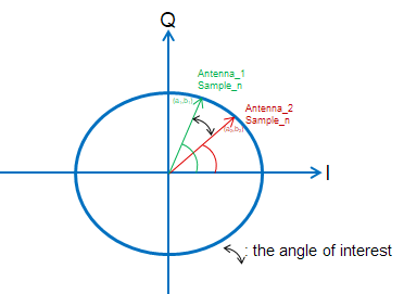
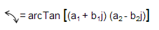
When the radio frequency wave incident on to an antenna array(assuming there are only 2 antennas on the board) and arrives at different antennas at different time, there will be phase difference between the antennas. So we extract the phase difference between ant1_sample[8 to 15] and ant2_sample[8 to 15]. The switch among antennas will cause measurement error, therefore we discard I/Q samples from 0 to 7 when calculating angles.
When using a custom HW with different antenna switch than what we have on BOOSTXL-AoA board, you might be able to use more I/Q samples if antenna switch settling time is shorter than 1 us. The method for determining how many I/Q samples can be used is explained in Valid I/Q Samples For Angle Calculation
The I/Q data can be presented into a X-Y domain with real number I and imaginary number Q (90 degree difference). As mentioned before, for each period of 250 kHz signal, we sample 16 I and Q data. If there is no difference, that means that the I/Q data is the same, therefore the phase between ant_1 sample1 will be the same to ant_2 sample1.
Here is the code putting I/Q data into 2 dimensions and then we passed the I/Q
pairs into function AOA_AngleComplexProductComp() to get final angle.
The reason for having a 32 offset for the sample array is that because the we use
8us as guard time(controlled by AOA_ANT_SWITCH_START_TIME). 8 us guard time
ith 4 MHz sampling rate gives us 32 samples, therefore we take the I/Q samples
after the guard time.
For users that want to have different guard time, the offset should be calculated as ‘guard time (in us) x sampling rate(in MHz)’.
Something to highlight is that in reality the 250kHz might not be perfect (for example, could be 255kHz or 245kHZ), therefore, there is slightly phase difference between ant_1 sample_n and ant_1 sample_(n + 16*1). Therefore run time compensation is also applied:
Because of the none perfect 250kHz tone, the phase difference is aggregated. Let’s say that every period will have 45 degree of delay. Then when comparing ant_1 sample_n and ant_1 sample_(n+16*1), the aggregated phase difference is 90 degree. But the real phase difference between every period is only 45. Therefore the calculated phase difference must be divided by the number of antennas used, in our case 2.
Valid I/Q Samples For Angle Calculation
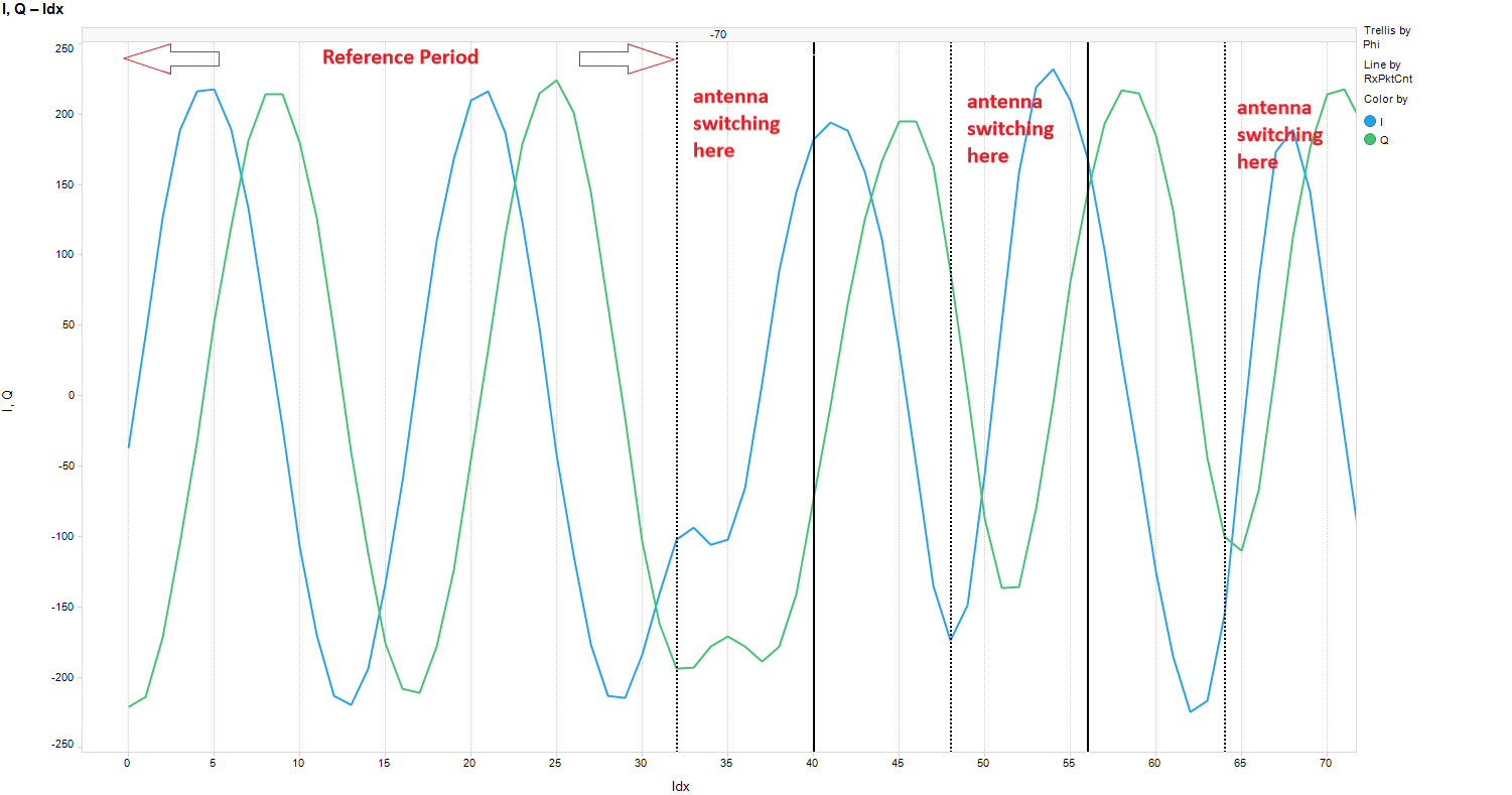
In order to determine what I/Q samples to use. The easiest way to tell is to plot all the I/Q samples.
The picture below shows the I/Q samples which were collected using the rtls_passive
example together with rtls_master and rtls_slave examples.
Table 21. Axis description¶ Axis Description X top Angle between a rtls_slave device and rtls_passive. X bottom Index number of I/Q data. Y I/Q values.
The first 32(index 0~31) samples are taken in reference period which there is no antenna switching. Therefore the I/Q plot looks like sinusoid wave.
After that at index 32, you can see when switching happened there comes discontinuity of I/Q samples.
Note
It’s easier to see the phase discontinuity when there is indeed phase difference. Therefore, before collecting I/Q data, make sure the angle between rtls_passive and rtls_slave is not 0 degree.
Angle Compensation
Under AoA_getPairAngles(), we will acquired the angle based on I and Q data. After that, angle compensation is added. Please see the code below. This is because angle estimation is affected by antenna pairs and frequency. The values p->gain, p->offset, channelOffset_A1 and channelOffset_A2 are based on lab measurements. Different antenna board design and frequency will give you different p->gain, p->offset, channelOffset_A1 and channelOffset_A2.
The following code can be found in AOA.c AoA_getPairAngles(), this is antenna pairs compensation.
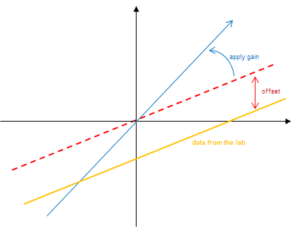
As you can see from the image above, the offset is applied to make sure the data received at 0 degree will derive 0 degree after the calculation and then the slope is changed to make it fit better with all the rest of the angles.
The compensation values for antenna array 1 can be found in
ant_array1_config_boostxl_rev1v1.c AoA_AntennaPair pair_A1[]
Followed by antenna pair compensation, we added frequency compensation.
For antenna array 1, the values used for frequency compensation can be found in
ant_array1_config_boostxl_rev1v1.c int8_t channelOffset_A1[40].
AoA Functions Overview
The functions covered under this section are all in AOA.c.
AOA_init:
For
rtls_passivedevice, this function takes care the following HW initialization.- Initialize GPIOs
- Set up I/O toggling patterns
- Route needed signal to DMA channels
- Set up GPTimer
For
rtls_slavedevice,AOA_initwill get the size of the RF override table.AOA_cteCapEnable:
For
rtls_passivedevice, it extracts the following 3 parameters which are input from users through NPI and then are stored in the RF RAM:- cteScanOvs: This is the I/Q sampling rate for the CTE. Table 22.
shows available values for this parameter. Out of box example is made with
cteScanOvs = 4. - cteTime: The length of the CTE. The allowed range is from 2~20 in 8us units.
The out of box is made with
cteTime = 20. This parameter in passive is used to calculate the number of available I/Q samples. - cteOffset: This gives the number of microseconds from the beginning of the CTE
to the sampling starts The allowed range is from 0~63. Out of box example is
made with
cteOffset = 4, which means the radio core will wait for 4us at the beginning of the CTE till it starts sampling. If this parameter is set larger than the actual CTE duration, thecteOffset = 4will be used.
For
rtls_slave, this function sets up the slave to send out CTE withcteTime*8usat the end of every connection packet by adding 1 extra override right before the end of the last override(0xFFFFFFFF).Table 22. cteScanOvs setting¶ Value Description 0 No special processing of AoA packet. 1 Process packets with AoA present in the header and sample CTE at 1 MHz.(not recommended, because this provides very little I/Q samples) 2 Process packets with AoA present in the header and sample CTE at 2 MHz. 3 Process packets with AoA present in the header and sample CTE at 3 MHz. 4 Process packets with AoA present in the header and sample CTE at 4 MHz. 15 Process packets with AoA present in the header but do not sample CTE. - cteScanOvs: This is the I/Q sampling rate for the CTE. Table 22.
shows available values for this parameter. Out of box example is made with
AOA_calcNumOfCteSamples
This function is only needed for
rtls_passivedevice to decide how big the array needs to be for I/Q samples and how many samples are avaiable per antenna. For example, if we take cteScanOvs = 4, cteTime = 20 and cteOffset = 4, then we should get ( cteTime*8 - cteOffset ) * cteScanOvs = 624 I/Q pairs. However, the radio RAM can only store upto 511 I/Q pairs. When this situation happens, the radio core will stop I/Q sampling once it fills up the radio RAM for I/Q storage area.AOA_cteCapDisable
For
rtls_passivedevice, this function will disable I/Q sampling and ignore AoA present in the header.For
rtls_slavedevice, this function will disable slave device to send out CTE.
AoA Application Overview
The steps to configure rtls examples to do AoA are described in the simplelink_cc2640r2_sdk_x_xx_xx_xx/examples/rtos/CC2640R2_LAUNCHXL/blestack/rtls_master/readme.html, please take a look at it when setting up the projects.
For users that are not familiar with editing predefined symbol/preprocessor symbol, please take a look at Accessing Preprocessor Symbols or Accessing Preprocessor Symbols
In the out of box software, the rtls_master and rtls_slave
will form a BLE connection. After
establishing the connection, rtls_master will send connection information
through UART to PC and then then node manager will pass this piece of
information to rtls_passive which can then track the connection.
Next, the node manager sets up AoA parameters for master and passive
and then master will send a packet over the air to slave
to setup the CTETime.
After that, the rtls_master will send a start AoA request over the air to
the rtls_slave and to rtls_passive over wire, then rtls_slave will
append CTE at the end of every connection packet.
rtls_passive can the do I/Q sampling and calculate angles base on the ConnectionCTE packets.
The sequence diagram below illustrates the whole process of how out of box examples work.
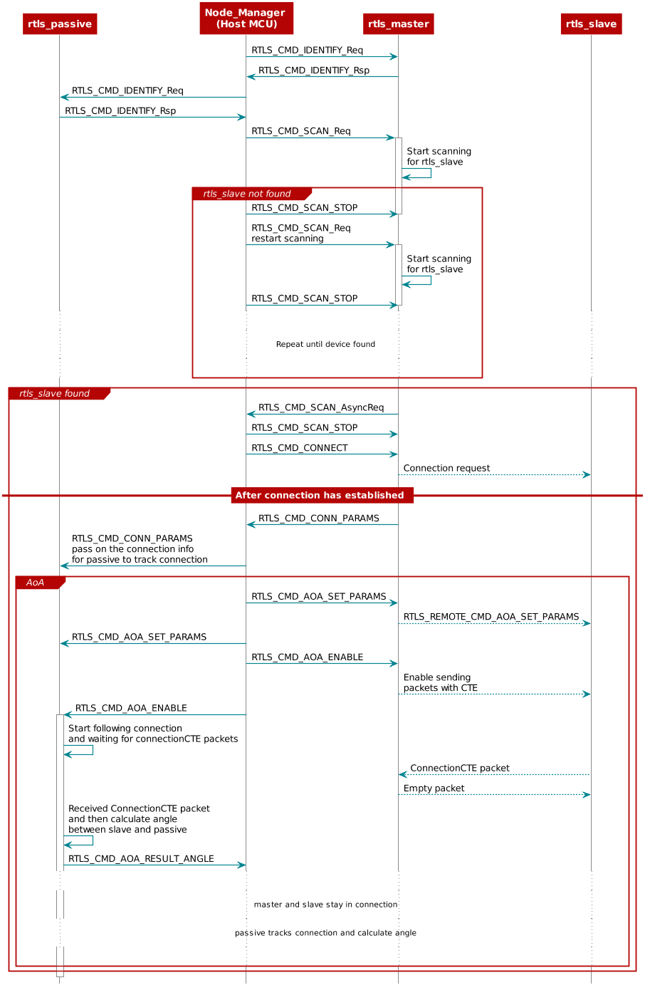
Figure 77. Setting up RTLS AoA network and enable AoA
Time of Flight
TI Time of Flight (ToF) is a proprietary technique used for secure range bounding by measuring the round trip delay of an RF packet exchange.
This is implemented in a Master-Slave-Passive configuration, where the Master sends a challenge and the Slave returns a response after a fixed turn-around time. The Master can then calculate the round trip delay by measuring the time difference between transmission of the challenge and reception of the response, subtracting the (known) fixed turn-around time. Passive will not participate in the exchange over the air, but will also measure the observed Time of Flight.
Due to the low-speed nature of the sampling clock frequency of the radio, when evaluated in the speed of light context, each individual measurement provides only a very coarse result. But by performing many measurements, typically several hundred within a few milliseconds, an average result with much better accuracy can be achieved.
Theory of Operation
Few things are faster than the speed of light, and that speed is known and constant at c. Electromagnetic waves propagate at the speed of light, and thus an RF packet propagates at the speed of light.
Since the speed is constant, this means that the time it takes for a wave to propagate is directly proportional to the distance. To find the distance to an object, we can record the time stamp when we transmit something and compare this to the time stamp when the reflection is received, divide by two and multiply by c. This is the operating principle of for example RADAR as well.
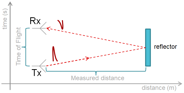
Figure 78. Reflected EM wave. If time between transmit and receive is t, then distance d is simply ct/2.
As opposed to RADAR, the reflector in TI ToF is considered active as it
does not reflect the outgoing signal meaningfully but instead must actively
send out the “reflection”.
There are at least two main challenges when doing this form of measurement:
- The time the reflector uses between receipt of the
PINGand transmission of thePONGwill affect the measured distance. - Light uses 3.3 ns to travel one meter, which means that the tick speed of a clock measuring the time of flight must apparently be at least 303 MHz to get 1 m spatial resolution.
The first challenge is overcome in the TI ToF solution by implementing a deterministic turn-around time in the slave/reflector device.
The second challenge is overcome by taking a statistical approach to measuring the distance. The frequency of the radio timer used to measure Time of Flight is 8 MHz, which means that the temporal resolution is 125 ns. The accuracy of the final measurement can be improved by oversampling the individual packet measurements. This is because there is jitter in the sample, and this jitter has a normal distribution. In order to achieve higher accuracy, the time of flight will be measured over many PING/PONG exchanges across multiple devices. Resolution is discussed further in the Resolution section and accuracy is discussed in the Accuracy section.
Terminology
PING: A packet sent to initiate a ToF measurementPONG: The response packet to a PINGRun/burst: A series of PING/PONG exchanges that are used to measure distanceTick: A single period of the RF core clock that is used to measure ToFSample: The measured RSSI, tick, and channel information for a single PING/PONG exchange
To recap, a ToF burst is a collection of PING/PONG exchanges. Each PING/PONG exchange results in a ToF sample which is a collection of RSSI, time stamp (in number of ticks), and frequency information. A burst can contain a configurable amount of PING/PONG exchanges and may operate on a configurable list of frequencies. At the end of a burst, all tick information can be averaged to form an estimate of distance. Information from multiple bursts across multiple devices can be combined to form a distance measurement within a given confidence interval.
Packet format
The modulation format is 2Mbps at 500kHz deviation using a piecewise linear shaper for the transitions. Packet content is based on a standard BLE packet with some modifications to meet the ToF use case.

The packets contain a random pre-shared sync word that is unique for each frame sent over the air, and that either side will be listening for in their RX cycle.
The syncword is how the RF circuitry detects that the packet is intended for the device, and also how the timestamps are generated for the measurements.
Packet Types
There are two types of packets that will be sent by the RF core when performing Time of Flight:
- Measurement packets: These are used to perform secure distance measurement
- Broadcast packets: These are used to synchronize passive nodes, and are not used for distance measurement
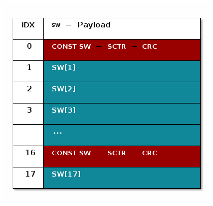
Measurement packets will use a random syncword that is generated using the Security module, the payload field of these packets is not used. Broadcast packets instead use a constant syncword and utilize the payload field to share synchronization information. The intent of the broadcast packets is to synchronize passive nodes. The concept of a passive node will be explained in the following section. The payload of a broadcast packet is shown below:

Note
Security in ToF is dependent on a good syncword generation algorithm. Syncwords should not be easily guessable by an attacker and should not be repeated. Instead they should be generated in a manner such that the trusted ToF nodes are able to determine the next syncword, but an attacker cannot. See Security. Since broadcast packets are not used for distance measurement, they may safely use constant syncwords.
ToF Roles
There are three roles supported by the ToF solution.
Master: Initiates ToF sequence by sending PINGSlave: Listens for PING, responds with PONGPassive: Listens for both PING and PONG
Master and passive will measure the Time of Flight using a timer in the RF core. While the passive role is not strictly required to run ToF, it will increase the robustness of the measurement by adding additional samples into the measurement and provide spatial diversity.
Since ToF is a statistical measurement, with more samples comes a higher degree of confidence in a given measurement. Passive nodes also add spatial diversity and can reduce the effects of reflections and multi-path fading in a ToF measurement. There is no limit to the number of passive nodes that can be added, but there must be at least one master and one slave.
The distance between Passive and Master must be known, so that this
distance can be calibrated out.
ToF Protocol
The Master and Slave devices will listen and transmit on a range of
frequencies provided by the application.
Meanwhile, the Passive device will listen to all the packets transmitted
between Master and Slave after they have achieved sync.
The Slave is initially in receive mode on the first frequency and is
listening for the first syncword SW0, this is the PING.
If the slave receives a matching packet in the initial listening period it
will send a PONG and will start following a time-slotted scheme where
it changes frequency and syncwords.
The master will send out a packet containing the first syncword(SW0) and some application defined payload. Immediately after this it will go into receive mode and wait for a slave to reply transmitting the second syncword(SW1) in the array.
Similarly, if the master receives a matching ACK/PONG packet in response
to the initial PING, it will follow the same time-slotted and frequency-
hopping scheme.
The passive will begin in RX mode, waiting for SW2
Once the Passive receives SW2, it will start following
the time-slotted and frequency hopping scheme.
Passive starts the radio timer when it receives SW2n, and then stops the
timer once Passive receives SW2n+1.
Periodically, the TOF Master will send out broadcast packets. Unlike measurement
packets, they use a constant syncword and contain a shared counter (SCTR)
embedded in the payload. The intent of the broadcast packets is to synchronize
the passive devices. The period of the broadcast packets may be configured
by changing tofBroadcast.period in TOF.c.
Note
Broadcast packets are not used for distance measurement.
![@startuml
participant "Master device" as Master
participant "Passive device" as Passive
participant "Slave device" as Slave
== Initial Sync ==
rnote over Passive
RX: waiting
for SW2
end rnote
Master -> Slave: SW<sub>0</sub> Freq<sub>0</sub> PING
activate Master
Master -> Master: SW<sub>1</sub>
Master -> Master: No Sync
deactivate Master
Slave -> Slave: Enter initial\nRX: SW<sub>0</sub> + Freq<sub>0</sub>
activate Slave
Master -> Slave: Tx: SW<sub>0</sub> Freq<sub>0</sub> PING
activate Master
Master -> Master: SW<sub>1</sub> RX
Slave -> Master: SW<sub>1</sub> PONG
deactivate Slave
deactivate Master
== Time-slotted ==
note over Master, Slave
From here the devices will go to the next
channel even if no sync is received.
end note
Slave -> Slave: SW<sub>2</sub> + Freq<sub>1</sub> RX
activate Slave
Master -> Slave: SW<sub>2</sub> Freq<sub>1</sub> PING
activate Passive
rnote over Passive
Start timer
end rnote
activate Master
Master -> Master: SW<sub>3</sub> RX
Slave -> Master: SW<sub>3</sub> Freq<sub>1</sub> PONG
rnote over Passive
Stop timer
end rnote
deactivate Slave
deactivate Master
deactivate Passive
loop
Slave -> Slave: SW<sub>n</sub> + Freq<sub>m</sub> RX
activate Slave
Master -> Slave: SW<sub>n</sub> Freq<sub>m</sub> PING
activate Passive
rnote over Passive
Start timer
end rnote
activate Master
Master -> Master: SW<sub>n+1</sub> RX
Slave -> Master: SW<sub>n+1</sub> Freq<sub>m</sub> PONG
rnote over Passive
Stop timer
end rnote
deactivate Slave
deactivate Master
deactivate Passive
end
group Broadcast Packet
activate Master
activate Passive
activate Slave
Master -> Slave: SW<sub>const</sub> Freq<sub>m</sub> [SCTR CRC]
deactivate Slave
deactivate Passive
deactivate Master
end group
loop
Slave -> Slave: SW<sub>n</sub> + Freq<sub>m</sub> RX
activate Slave
Master -> Slave: SW<sub>n</sub> Freq<sub>m</sub> PING
activate Passive
rnote over Passive
Start timer
end rnote
activate Master
Master -> Master: SW<sub>n+1</sub> RX
Slave -> Master: SW<sub>n+1</sub> Freq<sub>m</sub> PONG
rnote over Passive
Stop timer
end rnote
deactivate Slave
deactivate Master
deactivate Passive
end
...
@enduml](../_images/plantuml-2d6aacee3fd4049d2faf72c38c82f695b8a39b1c.png)
Figure 79. ToF measurement-burst sequence
If we consider the timing of the packets, we can try to illustrate the time of flight as the distance between the two first vertical lines below.
You can see that the internal clocks of the two devices are not synchronized, illustrated by the top line for each device, and you can see the three phases of a ToF measurement:
- Master sends PING, Slave receives
- Devices switch RF roles, TX to RX and RX to TX
- Response PONG is sent
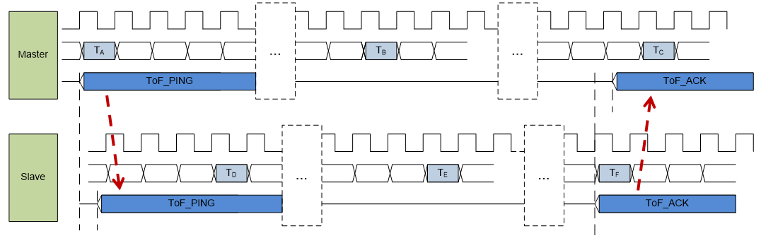
Figure 80. ToF Timing diagram. See legend below.
Resolution
Distance in ToF is measured in ticks of the radio timer, which runs at 8MHz. These tick values must be converted to meters in order to estimate the distance to the slave. The distance equation is used to perform the conversion. This section seeks to show step-by-step derivation of the tick to meter conversion constant.

Since ToF packets are EM waves, their propagation rate is fixed at c,
the time it takes for light to travel one meter. The result must be
divided by 2 since the time accounts for the round trip travel time of the
packet which is 2x the actual distance.
In order to convert tick values into time, they must be divided by the frequency of the RF core timer. Substituting this into the distance equation above gives the scaling factor used to convert ticks into meters.
![\begin{align*}
\begin{split}
\text{distance} &= \frac{1}{2}\times\text{t}\times\text{c}\\[16pt]
&= \frac{1}{2}\times\frac{\text{tick}}{8\si{\mega\hertz}}\times\text{c}\\[16pt]
&= \frac{\text{tick}}{2\times8\times10^{6}\text{s}^{-1}} \times 3\times10^{8}\si{\meter/\second}\\[16pt]
&= 18.75\si{\meter}\times\text{tick}
\end{split}
\end{align*}](../_images/math/1abcea4791d74fc4b5ceaac4f74f7c9f37b581b1.svg)
A ToF packet will travel 18.75 meters per tick. In software, this constant
is referred to by TICK_TO_METER. To convert a tick value to meters simply
multiply by TICK_TO_METER.
Accuracy
There are two physical phenomena that contribute to the derivations below:
- Jitter and phase noise in the clocks and oscillators inside the device
- Synchronized clocks between the devices performing ToF (e.g. master and slave)
Inside the RF core of the CC2640R2F there is a component called the correlator. The correlator is responsible for measuring the correlation value between two syncwords. When the RF core is running a ToF command, the correlator is responsible for starting and stopping the timer that measures ToF ticks.
The various devices in the ToF topology do not have a method for synchronizing their clock, and therefore there is some inherent random offsets between the symbol clocks in the transmitter and receiver. This means that over multiple ToF samples the time at which the correlator reports sync will drift slightly. This is illustrated by the gif below.
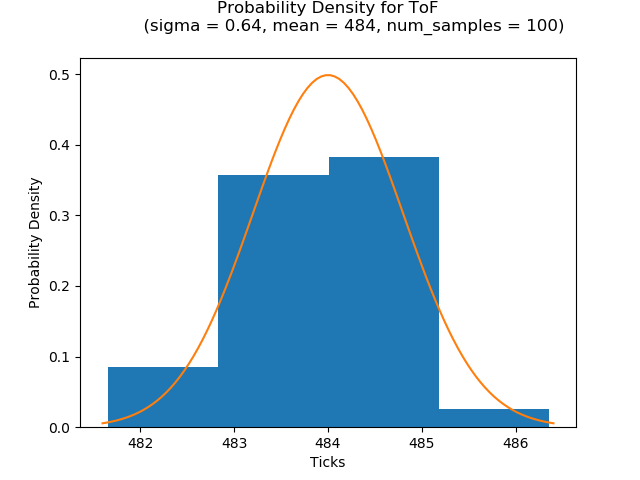
It is the correlator that is responsible for starting and stopping the timer that reports ToF ticks. Phase noise causes spreading in the “sync found” point in time and thus spreading occurs in the ToF results. Spreading in the sync found point causes ToF results to be spread across neighboring tick values. The variance has been observed by TI to be approximately 0.64.
The various devices in the ToF topology do not have a method for synchronizing their clock, and therefore there is some inherent offset in the clocks in comparison to each other. Spreading in tick values will not be synchronized between the devices performing ToF. Ultimately this means that results will be spread across 3-4 tick values for the entire system.
For a statistically significant set the distribution of ticks in the system can be approximated to a normal distribution and the true value is the mean value. An example histogram of ticks from a ToF run are printed below with the probably density function overlaid.
Let’s use a concrete example from a ToF run with slightly more samples, for example 7400. Plotting ToF results as a histogram for a given distance and number of samples yields results similar to the figure below.
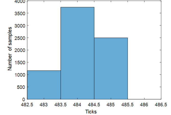
Using a concrete example based on the histogram above, we have the following results:

In the true distance calculation, we must account for calibration.
Calibration will be covered in depth in the Calibrate section.
For now, assume the calibration value is measured in ticks and is 484.

Plugging in the results from the histogram above results in
![\begin{align*}
\begin{split}
\text{$tick_{avg}$} &= \frac{\text{$count_{483}$}\times483}{count_{total}} + \frac{\text{$count_{484}$}\times484}{count_{total}} + \frac{\text{$count_{485}$}\times485}{count_{total}}\\[16pt]
&= 484.1756757
\end{split}
\end{align*}](../_images/math/2726168712dd048ee755b74e2d71a11f71f0b1cf.svg)
Plugging in the tick_avg to the final equation yields the following:

This example demonstrated the concept that ToF becomes more accurate with increased sample number. It also shows how ToF can be used to measure distances of less than 18.75m thanks to the spreading introduced by un-synchronized clocks between devices and phase noise/drift in the individual devices.
The general idea is that with more samples it is possible to achieve a narrower confidence interval at a given confidence level. Please see the calculator and write-up in the ToF SLA: Accuracy and Confidence Intervals Section www.ti.com/simplelinkacademy
ToF Time Slot and Frequency Hopping
Time of Flight can operate over multiple frequencies, performing frequency
hopping. A list of frequencies and a hop interval must be agreed upon by all
devices before starting ToF measurements. CMD_FS is used to program the
frequency synthesizer (FS) to the given frequency.
A coarse calibration of the frequency synthesizer must be done before the first
ToF_run() and is recommended to be redone every hour. Opening and closing
the ToF driver will trigger a coarse recalibration.
For more information, see TOF_calibrateSynth()
Once coarse calibration is complete, the CMD_TOF will handle the fine
calibration on the middle frequency inside the RF core. It is not required to
invoke CMD_FS before running CMD_TOF. A ToF command can be
broken down to two parts
- Fine FS calibration: 120us
- ToF measurement: 400us
This results in a time slot of 520 us when first hopping to a new channel and 400 us for the remaining measurements on that channel. It is recommended to perform ToF over multiple frequencies as multi-path fading is frequency dependent.
The frequency synthesizer is also pre-calibrated once during the very first run
after calling TOF_open() and the calibration values are stored.
Link Quality Indication (LQI) and Multi-path Filtering
Constructive interference caused by multi-path fading can result in very high LQI measurements. Measuring ToF on a multi-path reflection is undesirable as it is not an indication of the true distance. (non direct path). In summary, very high valued LQI measurements generally indicate that the packet has been affected by multi-path.
The ToF RF patch includes a parameter to ignore packets with LQI too high as a slave. Furthermore, it enables the ability to export LQI results for the master and passive.
Thus are types of filtering on LQI that are performed:
- RF core on the
ToF slave: packets with LQI above threshold are not responded to- Application core on ToF
MasterandPassive: local measurements with LQI above threshold are discarded
The RF core LQI filtering on the slave node can be configured by the
lqiThreshold parameter of the ToF command. This can be set from the
application core via the slaveLqiFilter RTLSCtrl parameter.
The application core LQI filtering is implemented as part of
TOF_getBurstStat(). The threshold can be set by changing the
postProcessLqiThresh RTLSCTRL parameter.
In summary, LQI filtering is performed on the PING as well as the PONG
packets.
- Slave receives packet with LQI above threshold, it will not respond (results in timeout for that SW)
- PING/PONG completes successfully, but master or passive measure too high of LQI on the returned packet. This will be filtered out on the application core.
Hint
When LQI or magnitude difference filters are set too aggressively, the system may in fact filter out many of the samples during a burst. This may appear that there is no ToF connection, when in fact the samples are being filtered out. It is important to ensure that ToF results are still statistically significant, (i.e. enough samples were used to derive distance estimation) before using a burst.
You can use RTLS_CMD_TOF_RESULT_RAW to observe all samples without
filtering. See also Debug Statistics.
Another sign of multi-path interference is a disparity of the received
RSSI in the <<1>> and the <<0>> symbols. The modulation scheme used by the ToF
PHY is Frequency Shift Keying (FSK) and thus each symbol correlates to a
positive or negative frequency deviation from the carrier.
The affects of multi-path are frequency selective so they will affect the
<<1>> and the <<0>> symbols differently. The ToF patch can also output magnitude
difference ratios for the <<1>> and the <<0>> symbols for each ToF sample.
Filtering based on magnitude difference is realized in the application core as
part of TOF_getBurstStat(). The magnitude difference threshold can be
set by the postProcessMagnRatio RTLSCtrl command.
Ultimately, the use of properly set LQI and magnitude difference filters can counter act the negative affects of multi-path interference on ToF measurements.
Security
The security of ToF is based on the premise that an attacker is unable to guess the next syncword to be used in the ToF run. This means that syncwords must never be recycled. If an attacker can easily guess the next syncword, the system is susceptible to replay attacks.
Instead, a random seed is distributed to the ToF slave using an encrypted connection. This seed is distributed to ToF passive nodes using a serial connection.
This seed is then fed into the AESCTRDRBG algorithm to generate a new
table of syncwords. These syncwords are then used for ToF. In order to optimize
the use of the radio while generating a new syncword table, the syncword list
can be double buffered (depending on tofSecCfgPrms->bUseDoubleBuffer) so
that the security module can be generating new syncwords while the RF core is
consuming them.
When operating in double buffered mode, the TOFSecurity module operates
on chunks of TOF_SEC_DBL_BUFF_SIZE size. Double buffered mode reduces
the amount of contiguous RAM required to run a burst. This is the recommended
mode of operation. When using single buffered mode, the buffer size will be
the total number of syncwords.
Note
When using doubled buffered mode (default), it is recommended to set the
number of total syncwords to be a multiple of TOF_SEC_DBL_BUFF_SIZE
to fully utilize the double buffering scheme.
In summary, the TOF security module generates a sequence of pseudo-random
syncwords that cannot be guessed by attackers who do not know the seed.
The syncword changes for each PING and PONG packet that are used for
distance measurement. Broadcast packets use constant syncwords, but are not
used for measuring distance, and thus do not affect security.
Random seed
The random seed is generated using the True Random Number Generator (TRNG)
hardware module and driver. This is distributed to via GATT profile.
The seed length is set by AESCTRDRBG_SEED_LENGTH_AES_128.
AESCTRDRBG
The syncword table is generated using AES-128 block algorithm based on
section 10.2.1.2 of NIST SP 800-90Ar1. This will use the TI-Drivers
AESCTRDRBG driver. See Driver API Reference for more info.
ToF Multinode Synchronization
As mentioned previously, the syncwords used by ToF must be constantly changing in order to prevent an attacker from guessing them. However, this presents a problem for the passive nodes which can miss a Time of Flight burst for the following reasons:
- Master/Slave miss the connection event
- Master/Slave fail to perform ToF
- Passive misses connection event
- Passive misses ToF
In all cases it is impossible for the passive node even though it has the security seed to determine which SW should be next.
This sychrnization issue is mitigated by the introduction of broadcast packets.
When the passive node loses sync, it will load its correlator with a
pre-determined constant syncword and begin looking for a broadcast packet.
The constant sycnword is hard coded on all nodes and set by TOF_CONSTANT_SW.
Broadcast packets are sent by the ToF master periodically during the ToF burst. These broadcast packets are potential passive sync points (PSP).
The format of the broadcast packet’s payload is described in
Packet Types. When a passive node receives a broadcast packet, it
will read the SCTR and compare it with its local counter to determine how
many PING + PONG exchanges it has missed and how far it must seek in its
table of generated syncwords. Once the passive knows how many packets it has
missed, it will know the next syncword to listen for and will have regained
synchronization.
The integrity of the SCTR is protected by a 16-bit CRC so the passive can
determine that it received the message correctly. The master is in charge of
updating the SCTR and sending broadcast packets.
The figure below shows a table of syncwords to be used by ToF with the PSPs/broadcast packets periodically appearing:
ToF Role Switching
The ToF role as discussed in this chapter of the User’s Guide is independent of
the RTLSCtrl role (e.g. rtls_passive, rtls_master, etc). This means that
it is possible for the rtls_passive to act as the ToF master and the
rtls_master to act as the ToF passive. This is a concept known as role
switching. Role switching improves system robustness through spatial diversity.
Spatial diverity is important because of multi-path reflections. If a given
node is currently appointed as ToF master, but is unable to measure a direct
path a role switch can occur and appoint a new node as master. The new master,
being placed at a different location has a chance of receiving the PONG
from the rtls_slave with a direct path.
Role switching is realized via an RTLSCtrl command. See RTLSCtrl for Time of Flight for more information about the command. It is recommended to monitor the statistics (e.g. number of okay samples) for each ToF node and appoint the node with the best results as ToF master for the next burst.
Role switching cannot be executed during a ToF burst and thus must be
coordinated in between invocations of TOF_run(...). If the command is
sent during a burst it will take affect on the next burst.
ToF Driver
The ToF driver is responsible for managing setting up the Time of Flight RF command, and interfacing between the RF driver and the application. Additionally, the ToF driver will use the ToF Security module to generate random seeds. Furthermore, the ToF Security module will use the random seeds for secure syncword generation using the Advanced Encryption Standard Counter Deterministic Random Bit Generator (AESCTRDRBG) algorithm.
From the application, it is relatively simple. You need to:
- Initialize
- Calibrate
- Run
- Collect the results
Initialize
The ToF driver needs a parameter struct with some information filled in. The example has this filled in already, but the most interesting parameters are:
tofRole- Device role: Master/SlavepT1RSSIBuf- Pointer to sample buffernumSyncwordsPerBurst- Number of syncwordspFrequencies- Pointer to array of frequenciesnumFreq- Number of frequenciespfnTofApplicationCB- Callback after runtofSecurityParams- Security configuration parametersfreqChangePeriod- How often should we change freq?syncTimeout- How long to wait for first sync wordpfnTofApplicationCB- Callback to applicationslaveLqiFilter- Automatic filtering for ToF Slave rolepostProcessLqiThresh- LQI threshold used for onchip post processingpostProcessMagnRatio- Magnitude radio threshold used for onchip post processing
The ToF driver is managed by the RTLSCtrl module, but its parameters and behavior are explained here to aide in understanding.
Run
When you call TOF_run(handle, tofEndTime) it will start immediately.
When combined with Bluetooth, you will get the time in Radio Access Timer
(RAT) ticks from the BLE Stack to use as ToF end-time.
Note
tofEndTime is measured in ticks of the Radio Access Timer (RAT) that runs at 4 MHz. It is important to remember that this is different than the RF core timer that runs at 8MHz that is used to measure ToF.
The tofEndTime parameter is valuable when scheduling ToF events in between stack communication such as Bluetooth.
Collect the results
This is done in the callback function given in the initialization parameters:
ToF_BurstStat tofBurstResults[TOF_MAX_NUM_FREQ] = {0};

void myCallback(uint8_t status) {
  TOF_getBurstStat(tofHandle, tofBurstResults);
  // Do something
}
This function takes the interleaved raw samples and averages them per frequency.

The raw samples are stored in a flat list (above), but the statistics function presents them per frequency:
typedef struct
{
    uint16_t freq;          // Frequency
    double   tick;          // Time of Flight in clock ticks, averaged over all valid samples for `freq`
    double   tickVariance;  // Variance of the tick values
    uint32_t numOk;         // Number of packets received OK for `freq`
} ToF_BurstStat;
The tick value can be converted to meters by subtracting the calibrated tick
value at 0 meters and multiplying with 18.75.
Calibrate
The measured Time of Flight will be longer than the actual Time of Flight. The error in measurement is caused by the following quantities:
- Slave turnaround time (switch from RX to TX)
- Intrinsic delay of device when using ToF PHY
These quantities are deterministic and non-zero. They differ slightly between devices based on the characteristics of the silicon. These characteristics will not change through the lifetime of the device, thus calibration must only be performed once per device and can be stored.
The following components make up a ToF measurement on master:

The following components make up a ToF measurement on passive:

Acting in a master role, each ToF measurement contains two delay components that should be calibrated for, the intrinsic delay of each device, and the turnaround time in the slave. Assuming a system of three devices, the master can be rotated to produce the following results, where M_12 denotes the ToF measured where device 1 is master and device 2 is slave. Note that below assumes ToF=0

Solving these equations results in the following:

Solving the above systems of equations gives the intrinsic delay of each device when operating as a master.
The same can be done for passive, keeping in mind that a passive measurement contains the delay from all three devices (master, slave, passive). For example with ToF=0. In the following equations, the following convention is used. P_123 represents as passive ToF measurement where is device 1 is passive, device 2 is master, and device 3 is slave. We will introduce a 4th device while calculating the passive delay, to show how the system scales as passive devices are added.

Rotating the passive role throughout the devices gives the following system of equations, note that here we are assuming that there are 4 passive devices. The method below can be scaled as more devices are added.

Solving this equation results in:

These delays should be measured in a controlled environment at production time in order to characterize the device, and should be stored in non volatile memory so that they can be used to adjust all ToF measurements.
In summary ToF calibration will results in a vector of tick values that should be expected on each frequency at a known distance for a given ToF role.
Application
The application has to somehow agree with the peer device(s) what frequencies should be used, the order of frequencies, and what the list of syncwords should contain.
In addition, it must call ToF_run(...) at appropriate times to initialize
the initial syncword search and the time slotted measurement burst.
This can also be shown as a (very) simplified sequence diagram. Note the below diagram doesn’t show any broadcast messages, but they will be inserted periodically:
![@startuml
participant BLEStack as stack
participant Application as app
participant ToF_driver as drv
participant ToFSecurity as sec
participant RF_driver as rf
participant Radio as radio
participant TRNG as trng
participant AESCTRDRBG as drbg
participant CryptoKeyPlaintext as crypto
activate app
app -> app : Initialize\nToF_Params
app -> drv : ToF_open(..)
activate drv
drv -> drv : Initialize
drv -> rf : RF_open(..)
drv -> sec : TOFSecurity_open(...)
sec -> trng : TRNGCC26XX_getNumber(...)
sec -> drbg : AESCTRDRBG_open(...)
drv -> drv : TOF_genSyncwordBatches(...)
app -> drv: TOF_genSyncWords(...)
drv -> sec: TOFSecurity_genSyncWords(...)
sec -> crypto : CryptoKeyPlaintext_initKey(...)
sec -> drbg : AESCTRDRBG_getBytes(...)
drv -> app : ToF_Handle
deactivate drv
deactivate app
...
stack -> app : BLE-stack\n connection established
activate app
app -> drv : ToF_GetSeed(...)
activate sec
sec -> drv : seed[AESCTRDRBG_SEED_LENGTH_AES_128]
deactivate sec
deactivate app
deactivate trng
== Send random seed to ToF Slave \nvia encrypted BLE-Stack connection ==
activate stack
stack -> app : BLE-stack\n connection event ended
deactivate stack
activate drv
app -> drv : ToF_run(freqs, ...)
activate drv
drv -> rf : RF_schedCmd
deactivate drv
activate rf
rf -> radio : Load patch
activate radio
rf -> radio : Run command
radio -> radio : Search for\nsync
radio --> : SW<sub>0</sub>
radio <-- : SW<sub>1</sub>
radio -> radio : Loop \nand store timestamps
activate radio
radio -> rf : Interrupt
deactivate radio
alt RF_EventRxOk
rf -> drv : RF_Callback(RF_EventRxOk)
drv -> drv: update SCTR, setup next broadcast message
drv -> drv: TOF_genSyncwordBatches(...)
drv -> drv: TOF_genSyncWords(...)
drv -> sec: TOFSecurity_genSyncWords(...)
sec -> crypto : CryptoKeyPlaintext_initKey(...)
sec -> drbg : AESCTRDRBG_getBytes(...)
drv -> app : Callback
else RF_EventDoubleSyncWordBufferSwitch
rf -> drv : RF_Callback(RF_EventDoubleSyncWordBufferSwitch)
drv -> drv: TOF_genSyncwordBatches(...)
drv -> drv: TOF_genSyncWords(...)
drv -> sec: TOFSecurity_genSyncWords(...)
sec -> crypto : CryptoKeyPlaintext_initKey(...)
sec -> drbg : AESCTRDRBG_getBytes(...)
drv -> radio: New syncword buffer ready
else RF_EventRxNOk
rf -> drv : RF_Callback(RF_EventRxNOk)
alt if Passive
drv -> drv: TOF_handleOutOfSync
end
drv -> drv: TOF_genSyncwordBatches(...)
drv -> drv: TOF_genSyncWords(...)
drv -> sec: TOFSecurity_genSyncWords(...)
sec -> crypto : CryptoKeyPlaintext_initKey(...)
sec -> drbg : AESCTRDRBG_getBytes(...)
end
deactivate rf
== In application CB ==
activate app
app -> drv : ToF_getBurstStats(..)
drv -> drv : Calculate stats\nfrom timestamps
drv -> app : ToF_BurstStats
app -> app : Average a bit
[<- app : Display
@enduml](../_images/plantuml-60643ea243763a1202f7dfd0d4262f0d7bd9e57a.png)
Figure 81. ToF Application Example
Debug Statistics
The ToF driver contains a feature where it can track statistics over the
multiple ToF measurements. These statistics are stored in a global structure
(gTofStatistics) that may be added to the debug live watch view in the IDE.
Statistics tracking is enabled by throwing the RTLS_TOF_DEBUG define.
RTLSCtrl for Time of Flight
The previous sections of this guide described the theory of Time of Flight, its RF Core functionality, as well as its low level driver and security module.
This section aims to describe the remote procedure calls and parameters related to Time of Flight that are exposed via the RTLSCtrl interface. See General RTLS Software Architecture for an overview of how RTLSCtrl fits into the TI RTLS software architecture.
ToF Parameters
The behavior of ToF is controlled via the RTLS python environment parameters set
in the RTLS_CMD_TOF_SET_PARAMS UNPI request. This request is sent to the
master and passive nodes. The master will relay the selected ToF settings to the
slave over BLE. RTLS_CMD_TOF_SET_PARAMS must be called before running ToF.
See rtlsTofParams_t for more information.
ToF Result Mode
The RTLS nodes can be configured to report ToF sample data in the following ways:
| ToF Result Mode | Summary | Number of serial frames/burst | Payload Information |
|---|---|---|---|
RTLS_CMD_TOF_RESULT_DIST |
Provides a single distance estimation across all frequencies in the burst and moving averaged across all bursts | 1 |
|
RTLS_CMD_TOF_RESULT_STAT |
Provides tick average and variance per frequency | 1 for each frequency used |
|
RTLS_CMD_TOF_RESULT_RAW |
Provides each tick sample within the burst directly from the RF core. | numSyncwordsPerBurst/2 |
|
ToF mode can be controlled via the resultMode field of
RTLS_CMD_TOF_SET_PARAMS. Result modes lower in the table provide more data to
the PC, but also require the embedded device to send UNPI frames more frequently
and use more RAM.
Attention
It is recommended to use the most verbose mode to prototype ToF algorithms on PC and then reduce the frequency at which data is sent by balancing the processing between the node manager and embedded devices.
ToF Run Mode
runMode is a parameter within the RTLS_CMD_TOF_SET_PARAMS that describes
what will trigger ToF measurements to be taken and how frequently ToF measurements
will run.
It is important to consider power budget when selecting a runMode. Continuously running ToF is good for prototyping algorithms on the PC side as a lot of data is provided, but is not the most efficient for battery powered operations. It is recommended to trigger ToF based on RSSI and only run to collect the minimum number samples required to achieve a given confidence interval.
| ToF Mode | Summary |
|---|---|
TOF_MODE_CONT |
ToF will run continuously until RTLS_CMD_TOF_ENABLE
is called with the stop parameter |
TOF_MODE_AUTO |
ToF is automatically triggered based on RSSI of the
slave device The RSSI is measured during the connection
event and the threshold is set by the autoTofRssiThresh
parameter of RTLS_CMD_TOF_SET_PARAMS |
Syncwords Per Burst
Another parameter of interest in the RTLS_CMD_TOF_SET_PARAMS command
is the number of samples. numSyncwordsPerBurst dictates how many
syncwords are used by each ToF burst. It takes two syncwords to create a
single ToF sample (PING + PONG). This yields the following equation:
NumTickMeasurements = numSyncwordsPerBurst/2 - numPSPs
Put another way, the number of tick measurements performed per time of flight
burst is half of the numSyncwordsPerBurst parameter minus any passive
sync points (PSP) that are included in the burst. The period
of the PSPs are defined by the fields in the broadcast structure
RF_cmdTof.BC of the ToF command. By default, there is one PSP per batch
of syncwords from the AESCTRDRBG.
(set by gTofSecHandle.numOfSyncWordsPerBuffer)
Note
Remember that not all ToF modes report out the raw tick values of each sample.
This means you might not observe more data being sent to the PC when increasing
numSamples. This is because in modes like RTLS_CMD_TOF_RESULT_DIST and
RTLS_CMD_TOF_RESULT_STAT there is some preprocessing of the samples performed
on the device.
Frequencies
RTLS_CMD_TOF_SET_PARAMS also takes a frequency list and number of frequencies.
Each entry in the frequency list corresponds to a channel that Time of Flight
should be performed on. It is important to have diversity in the frequencies
selected for ToF as Physical factors such as multi-path fading are frequency
selective.
frequenciesis a list of frequencies in MHz of the BLE channels to use for ToFnumFreqis the number of channels in this list
BLE channels are spaced 2 MHz apart and range from [2402, 2480] (inclusive). While ToF does not use the BLE physical packet format directly, it does use the same channel map. Frequencies in this range are acceptable ToF parameters. A channel is specified by the frequency of its carrier wave.
The frequency list can be initialized in Python using the code below:
tofFreqList = [2408, 2412, 2418, 2424] #Other options: 2414, 2420
tofNumFreq = len(tofFreqList)
LQI Filters
As discussed in Link Quality Indication (LQI) and Multi-path Filtering, there are two configurable LQI filter values that affect the master/passive and slave LQI processing respectively. See the table below for each parameter and description of its use:
| RTLSCtrl Parameter | Description | Range |
slaveLqiFilter |
If the slave receives a PING with LQI greater than this threshold, it will not respond | 0-255 |
postProcessLqiThresh |
If master or passive receives a measurement with LQI greater than this, it will be discarded | 0-255 |
Magnitude Ratio Filter
Another signature of multi-path interference is a disparity between the RSSI
of the <<1>> and the <<0>> symbols. The RF core will report the magnitude of
the <<1>> and the <<0>> symbols as part of the ToF results, and
the results will be post processed in TOF_getBurstStat(). The ratio of
sym1/sym0 and sym0/sym1 will be calculated as a floating point double.
If either of the ratios is greater than postProcessMagnRatio/100.0 then the
result is discarded.
Role Switch
The benefits of role switching and its theory are described in
ToF Role Switching. This section describes the RTLSCtrl that realizes
role switching namely RTLS_CMD_TOF_SWITCH_ROLE. The command takes a single
8-bit parameter which is an enumeration of the new role. As described
previously, it is only valid to switch roles from master to passive and vice
versa. Role switching may occur independently of setting ToF parameters.
The role switch command will do validation on the state change and then set
RF_cmdTof.bMaster accordingly. Note that role switching cannot occur within
a ToF burst, and must be coordinated across master and passive between bursts.
Valid ToF roles are defined in TOF.h::ToF_Role.
Calibration
As discussed in Calibrate a calibration vector for ToF must
consist of the following: Role, Frequency, distance, and Tick average.
Calibration is a method for measuring and storing the tick average for a given
frequency, role, and distance. All frequencies are calibrated at the same
distance as set by the calibDistance parameter of the
RTLS_CMD_TOF_CALIBRATE command. The calibration procedure consists of
taking a moving average over enough runs to produce the number of samples per
frequency as specified by the samplesPerFreq parameter of the command.
The command has the following request and response types:
SyncReq: Sends request to node to begin calibrationSyncRsp: On validation of parameters and calibration start, return statusAsyncRsp: OncesamplesPerFreqhave been stored for each frequency, return calibration vector.
The calibration command will behave as follows:
useCalibFromNV== True and calibration exists in NV, no action, return immediatelyuseCalibFromNV== True and calibration doesn’t exist in NV, begin calibration, perform moving average over ToF bursts untilsamplesPerFreqis reached. Store result andcalibDistanceuseCalibFromNV== False will perform calibration regardless of whether it it exists in NV or not. The results will be stored in NV.
The Calibration command follows Using Simple NV for Flash Storage. It will use the OSAL SNV to store the calibration. This is because of the added benefit that OSAL SNV implements EEPROM emulation and allows the calibration to be overwritten without erasing the whole page.
The NVID used by the TOF calibration start at BLE_NVID_CUST_START and
use the following number of NVIDs :
1 + (calibParams.numFreq / RTLS_TOF_FREQ_PER_NV_BLOCK) + (calibParams.numFreq % RTLS_TOF_FREQ_PER_NV_BLOCK)
The calibration procedure will use the first NVID to store meta-data about the
calibration including frequency list and calibration distance. The following
NVIDs are used to store ToF_BurstStat for each frequency’s moving average
as calculated during calibration.
The calibration vector can be read using RTLS_CMD_TOF_CALIB_NV_READ.
Warning
Calibration is role, frequency list, and device dependent. This means that if the ToF frequency list, role, or device is changed, calibration must be repeated.
Currently the calibration results are only used when in TOF_MODE_DIST,
however the same concept applies
(averaging over Tick values to establish a reference point for a known distance)
for all modes of operation. In RAW or STAT mode, calibration should be
calculated and stored on the PC.
Interleaving with Bluetooth
A Bluetooth LE device in a connection is bound to wake up and transmit or
receive at certain times known as Connection Events. The interval between
such events is called a Connection Interval.
The Passive device is integrated with connection monitor functionality,
therefore, it can obtain connection information(rssi, time stamp) and also
listens for ToF packets at the end of each connection event and providing
calculated distance.
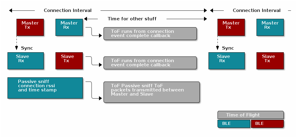
In the time between the end of one connection event and the start of the next scheduled connection event, there is time to schedule other RF commands, such as ToF.
The available time can vary, but a time stamp is provided in the connection event complete callback for when Time of Flight has to be finished using the radio.