Antenna Design

One of the most critical pieces of any product using mmWave radar is the antenna. The antenna design is critical for the overall performance, efficiency, and cost of the sensor system. There are several factors to consider when designing an antenna which can allow designers to maximize the achievable performance for their specific application. TI provides numerous different evaluation modules and reference designs, which give designers a resource that they can leverage as a starting point, or copy entirely if applicable. Figure 1 shows an example of the antenna design used on the IWR6843ISK, with its components labeled.

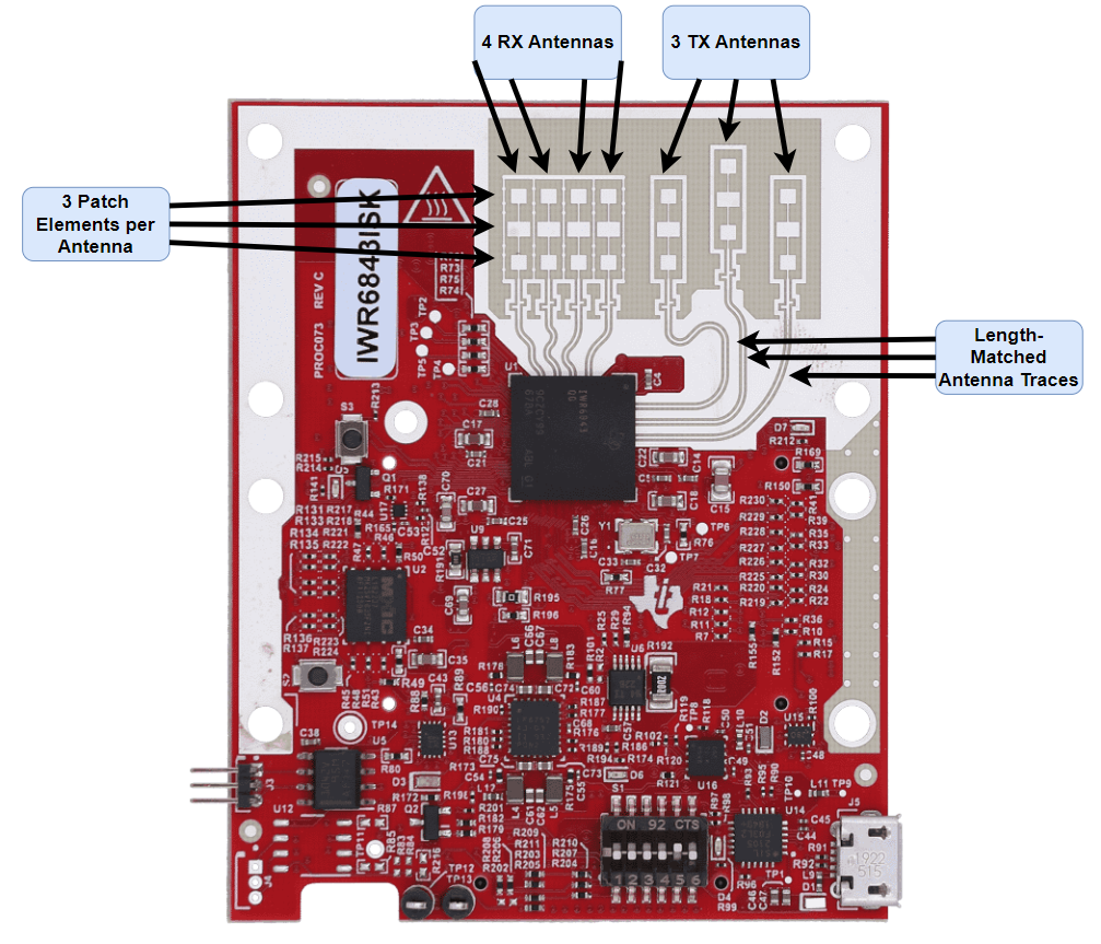
Figure 1. An IWR6843ISK with its antenna components labeled

Number of Antennas

Every mmWave radar sensor has a fixed number of transmitter (TX) and receiver (RX) antennas. When selecting the right radar device for an application, it is critical to consider the number of antennas provided and how that may affect performance. Increasing the number of TX or RX antennas will increase the number of virtual channels which the device has, which therefore will increase the angular resolution.

Virtual Antenna Array

A virtual array is a spatial arrangement of each TX-RX pair of an antenna array based on its position on the PCB plane. For ‘N’ number of RX antennas and ‘M’ number of TX antennas there will be ‘N x M’ number of virtual antenna elements. The coordinates of the virtual elements will be equal to the sum of individual coordinates of the TX-RX pair. So, the TX and RX antennas can be placed on the PCB at different positions and spacing to emulate different virtual antenna array patterns. Figure 2 shows two different antenna patterns available on TI evaluation modules for the IWR6843 radar sensor, where ʎ represents the wavelength of the center frequency being transmitted.

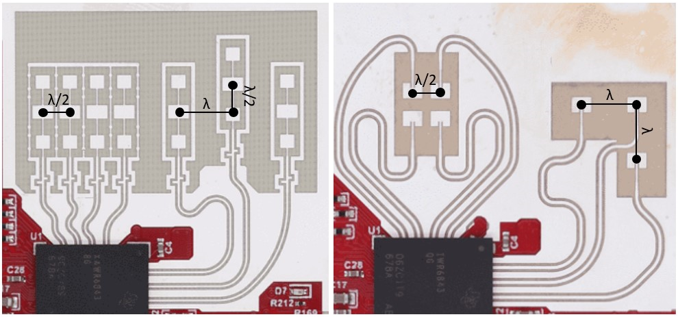
Figure 2. Antenna patterns used on the IWR6843ISK Evaluation Module(Left) and the IWR6843ISK-ODS Evaluation Module(Right)

While both antenna patterns utilize 3 transmitters and 4 receivers, they use different number of antenna patches as well as a different layout for the antennas, which will offer different performance tradeoffs. Figure 3 shows the corresponding virtual antenna arrays which are translated from the antenna patterns shown in Figure 2.

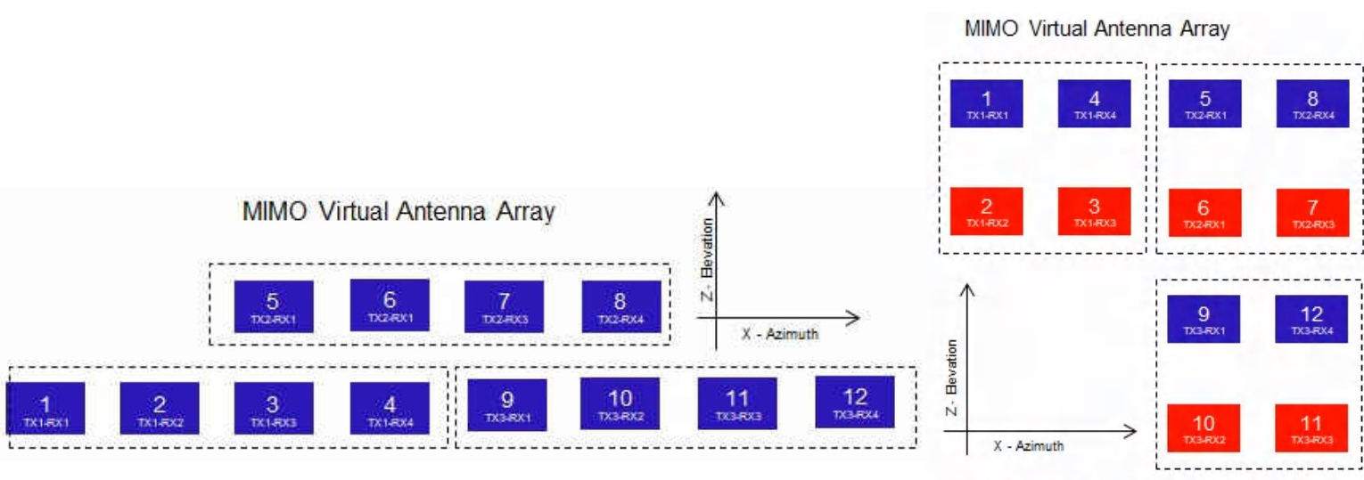
Figure 3. Derived virtual arrays for the IWR6843ISK Evaluation Module(Left) and the IWR6843ISK-ODS Evaluation Module(Right)

In the array on the left of Figure 2, TX1 creates virtual antenna elements 1, 2, 3 and 4 with the 4 RX antennas which are spaced by a distance of half wavelength (ʎ/2) on the azimuth plane. TX2 is spaced from TX1 by a distance of ʎ on the azimuth plane and ʎ/2 on the elevation plane. This has resulted in virtual elements 5, 6, 7 and 8 made with the 4 RX antennas which are at a distance of ʎ (azimuth) and ʎ/2 (elevation) from 1, 2, 3, and 4 respectively. Similarly, virtual elements 9, 10, 11, and 12 made from TX3 and 4 RX pairs are at a distance of 2ʎ (azi) from 1, 2, 3 and 4. This results in 8 virtual channel elements in the azimuth plane, and only 2 in the elevation plane. This means better angular resolution will be achieved in the azimuth plane than the elevation plane.

Similarly, the array on the right of Figure 2 shows a virtual antenna pattern having equal number of virtual elements in both the azimuth and elevation planes, which will provide equal point cloud density in both the azimuth and the elevation planes.

Antenna Spacing

RX-RX Spacing

Just as the number of Antenna elements hold a lot of importance and significance, the co-existence of them is equally important too. It is essential that the antennas do not influence the adjacent/neighbor elements performance due to coupling.

By principle, the phase difference between the reflected waves from an object falling on two different receiver antennas helps to calculate the angle of arrival of the object. Half wavelength spacing between RX antennas would enable the maximum unambiguous angle of arrival (90 degrees) estimation.

As discussed in the Fundamentals of FMCW Radar Module, the maximum theoretical field of view (FOV) that two antennas spaced L apart can service is represented by:

(1)\[\theta_{max} = sin^{-1}(\frac{\lambda}{2L})\]

Therefore, the maximum FOV is achieved when L = ʎ/2

TX-TX Spacing

When two transmitter antenna elements are excited together, their spacing will impact their mutual coupling and subsequently the effective radiation pattern. As the antenna elements are placed closer (less than ʎ/2), their fields interact more, resulting in lower gain and a wider FOV. As the spacing increases, the radiation pattern becomes more directed with increased gain and a lower FOV. Grating lobes start to appear as the spacing goes above ʎ/2, resulting in reduced efficiency. Therefore, ʎ/2 spacing is preferred (in both azimuth and elevation planes) for the optimal radiation pattern in the majority of use-cases. Figure 4 shows how the radiation pattern can be affected as the spacing is increased and decreased.

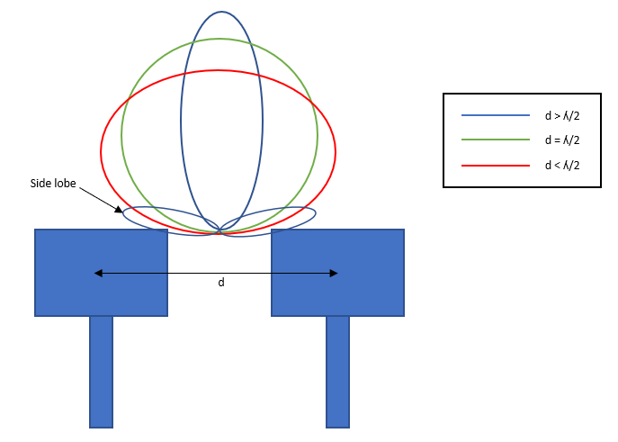
Figure 4. Antenna radiation patterns as the spacing between two antennas elements is changed

<–>

TX-RX Spacing

The distance between the transmitter and receiver channels is important as it determines the isolation between the channels. As the distance increases, the isolation will also increase which improves the signal integrity. If the RX and TX channels are very close, the TX power will leak directly into the RX and will distort the entire received signal, therefore reducing the signal-to-noise ratio (SNR). Additionally, this leakage can cause the receiver to start detecting false signals.

Patch Design

Patch antennas are one of the most common forms of antennas used in mmWave radar sensors. Each antenna can have one or more patches which will affect the performance of the antenna. As the number of patches used for an antenna element increases, the signal gets more focussed and directed, resulting in a higher gain at the expense of a lower field of view (FOV).

Number of Antenna Elements/Number of Patches in Single Element	Gain (dB)	FOV (Degrees)
Increase	Increase	Decrease
Decrease	Decrease	Increase

The distance d between the patches also impacts gain and FOV. It is typically kept at ʎ/2 for the optimal radiation pattern as shown in Figure 5.

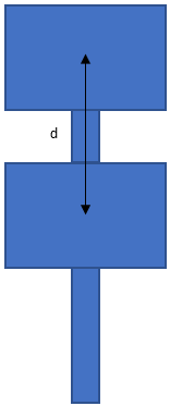
Figure 5. Example of a single antenna which utilizes two patches

Patch antennas consist of metallic structures printed on the PCB substrate, over a ground plane as shown in Figure 6. Each patch element connected to a transmitter radiates when the transmitter is excited.

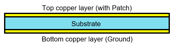
Figure 6. A visualization of the cross section of the relevant PCB layers to the patches

The dimensions of the patch depend on the center frequency of operation. In rectangular patches, the length and width will be ratios of the wavelength associated with the operating frequency. A higher the frequency of operation will result in a lower wavelength wavelength and thus utilizes a smaller patch, as shown in Figure 7. The patch dimensions will also be impacted by the thickness and dielectric values of the substrate.

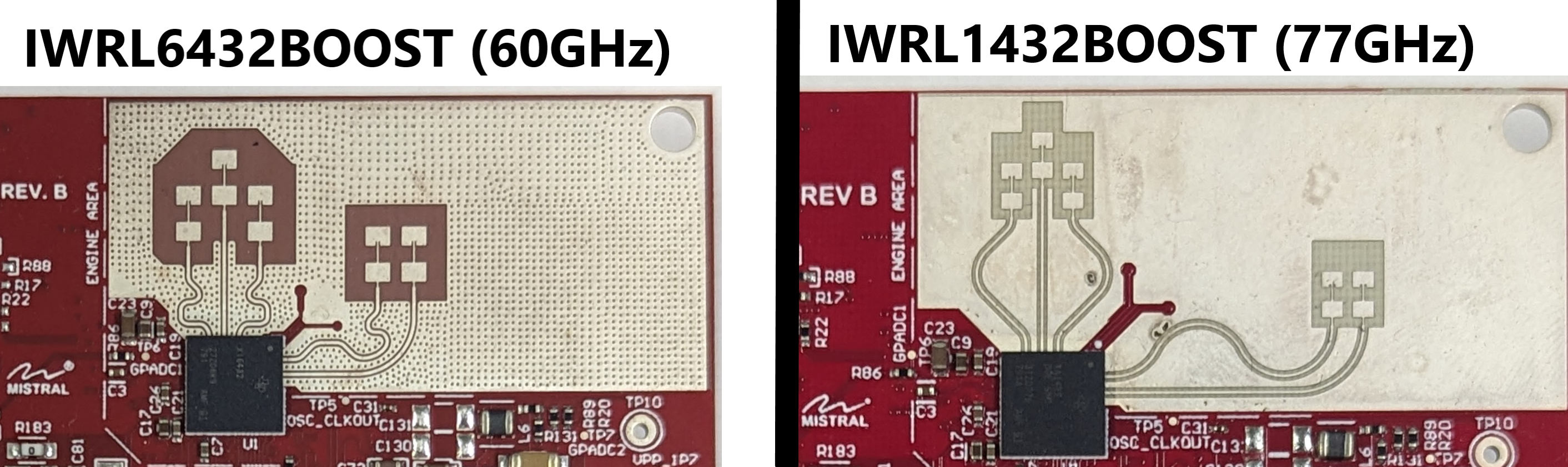
Figure 7. Comparison of the antenna area on the IWRL6432BOOST (Left) and the IWRL1432BOOST (Right). The patches on the IWRL1432BOOST are smaller and space closer together.

The patches are commonly fed via a microstrip transmission line which is usually of 50ohm impedance, determined by the width of the microstrip. The substrate properties will also impact the transmission line impedance which should be considered when calculating its width. For maximum power transfer, the impedance of the transmission line should match to that of the patch edge. This impedance match can be achieved using different methods such as inset feeding, using quarter wave transformer (QWT), or stub matching. Figure 8 shows an example of an inset fed patch antenna.

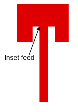
Figure 8. An example of an inset fed patch antenna

Antennas of the same type (TX or RX) should also have feed lines of the same length to ensure that the signal propagation time (and any delays it causes) are coherent across the MIMO array. The direction that antennas are fed from also affects their polarization, but this can typically be adjusted for via software.

Impact of Substrate

The PCB material properties such as dielectric constant, loss tangent, and thickness affect the antenna design. The higher the dielectric constant the smaller will be the antenna size but the bandwidth and efficiency might reduce. High loss tangent values will reduce antenna efficiency by increasing the dissipation of RF energy as heat. Thickness of the substrate impacts the size of the patch and in turn the input impedance of the patch. Thus, substrate properties also affect the impedance matching of the patch.

Dielectric Constant/Loss Tangent	Bandwidth	Efficiency
Increase	Decrease	Decrease
Decrease	Increase	Increase

Summary

• The antenna pattern can be designed to produce an array of virtual elements that optimizes performance according to application requirements

• A radar with an array of a greater number of elements will produce detections with better angular resolution

• Half wavelength spacing between RX antennas enable the maximum unambiguous FOV of 90 degrees

• An individual antenna element can be designed with more patches to increase the directionality of the signal

• PCB material with low dielectric constant and loss tangent values are preferred for better antenna performance