6.5) Fully Convolutional Networks for Predictive Maintenance with Time-Series Data

### Introduction In this module, we will look at a predictive maintenance application with sensor inputs. Predictive Maintenance relies on sensor signals to monitor health condition of the machine and also make predictions on the health status in the future. Sensors typically output one-dimensional time-series data such as Accelerometer data (vibration), acoustic data, electric current signals and ultra-sound data. Fully Convolutional Networks (FCNs) are very powerful deep learning techniques for Time Series Data especially when labelled data is available. You can watch our webinar for more detailed explanation in a presentation format <a href="https://training.ti.com/process-edge-ai-goes-mainstream-industrial-applications" target="_blank"> at this link.</a> You can download the full code base from <a href="https://e2e.ti.com/support/processors-group/processors/f/processors-forum/1042876/faq-sk-tda4vm-jacinto-october-monthly-webinar-edge-ai-goes-mainstream-in-industrial-applications?tisearch=e2e-sitesearch&keymatch=webinar#" target="_blank"> this E2E forum link. </a> This code base has all the Jupyter notebooks referenced in this module. **Step 1:** Develop the CNN model using a given dataset on a PC. Jupyter notebook to use: 1_create_model_Timeseries_FCN.ipynb **Step 2:** Benchmark and compile the model on the TI Cloud Tool Jupyter notebook to use: 2_compile_model_CLOUD_TOOL_PM_FCN.ipynb **Step 3:** Deploy the model on the Edge AI Starter Kit EVM Jupyter Notebook to use (On Starter Kit EVM): 3_deploy_model_SK_EVM_PM_FCN_ARM_ONLY.ipynb Jupyter Notebook to use (On Starter Kit EVM): 3_deploy_model_SK_EVM_PM_FCN_DL_ACC.ipynb These three steps will be described in detail in this module. <hr> ### Prerequisites Prerequisites for both hardware and software are the same as [prerequisites for module 6](./6_end_to_end_ai.html#prerequisites). If you plan to run step1 of this module which is creating the CNN model, you will need to have Anaconda Jupyter setup as described in [module 4.](./4_hello_ai.html#sw-installation) You can also choose to run this completely on the Edge AI cloud tools if you do not have Edge AI starter kit yet. This example uses tensorflow package for Step 1 so please make sure to install this using the command below on the PC. 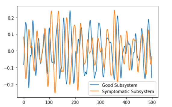<hr style="width:50%; margin: auto;" /> ```c pip3 install tensorflow ``` <hr style="width:50%; margin: auto;" /> ### Step 1: Develop the CNN model using a given dataset Jupyter notebook to use (On PC): 1_create_model_Timeseries_FCN.ipynb The dataset we are using here is called FordA which has 3601 training instances and another 1320 testing instances. Each timeseries corresponds to a measurement from an automotive subsystem. Each time series data is either from a good subsystem or one that is symptomatic. This is a binary classification task. Below is one timeseries data example for each class in the dataset where time is represented in the x-axis. ![MV CNN Model](./resources/6_5_data_set.png) Next step is to train the model similar to the process described in module 6.4. This process is time consuming and typically, this is done on high performance systems. For this simple application, you should be able to run on your local PC. Time series sensor data is available for both good and symptomatic automotive subsystems so it will be a binary classification problem. We can use state of the art Fully Convolutional Networks to solve this problem. Below code snippet is used to create the model in Keras and Tensorflow framework. ``` model = Sequential() model.add(Conv2D(filters=64, kernel_size=(1,3), activation='relu', padding='same', input_shape=rawData_train_FCN.shape[1:])) # Layer1 model.add(Conv2D(filters=64, kernel_size=(1,3), activation='relu', padding='same')) # Layer2 model.add(Conv2D(filters=64, kernel_size=(1,3), activation='relu', padding='same')) # Layer3 model.add(GlobalAveragePooling2D()) model.add(Dense(1, activation='sigmoid')) # Layer4 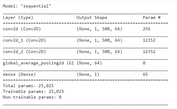model.summary() ``` We can see the overall model with multiple layers as shown in the below Figure. ![MV CNN Model](./resources/6_5_model_arch.png) ### Step 2: Compiling the model using open source runtime libraries Jupyter notebook to use (On Edge AI Cloud Tool): 2_compile_model_CLOUD_TOOL_PM_FCN.ipynb Once the Tensorflow lite model is created in Step 1, the next step is to compile the model similar to steps 2 and step 3 in Hello world example of module 4. The model compilation needs to happen on a host PC and the cloud tool is an option. You can reuse many Jupyter notebook examples provided for compilation. Also, as described in module 5, there are multiple options to optimize the compile process. Below code snippets show the compilation procedure and the overall jupyter notebook has the complete code that you can use directly. ```c # create the output dir if not preset # clear the directory os.makedirs(output_dir, exist_ok=True) for root, dirs, files in os.walk(output_dir, topdown=False): [os.remove(os.path.join(root, f)) for f in files] [os.rmdir(os.path.join(root, d)) for d in dirs] tidl_delegate = [tflite.load_delegate(os.path.join(os.environ['TIDL_TOOLS_PATH'], 'tidl_model_import_tflite.so'), compile_options)] interpreter = tflite.Interpreter(model_path=tflite_model_path, experimental_delegates=tidl_delegate) interpreter.allocate_tensors() input_details = interpreter.get_input_details() output_details = interpreter.get_output_details() for num in tqdm.trange(5): interpreter.set_tensor(input_details[0]['index'], test_FCN) interpreter.invoke() ``` As we discussed in modules 4 and 5, this step produces the artifacts used by TI's deep learning accelerator. The cloud tool can also be used to benchmark the model performance. When you run the provided notebook, it will give you inference results and performance information. The next step is now to deploy this model to the actual hardware. ### Step 3: Deploying the machine vision inference on the edge AI device Jupyter Notebook to use (On Starter Kit EVM): 3_deploy_model_SK_EVM_PM_FCN_ARM_ONLY.ipynb Jupyter Notebook to use (On Starter Kit EVM): 3_deploy_model_SK_EVM_PM_FCN_DL_ACC.ipynb The deployment function is primarily inference function using the artifacts generated in step 2. After your code development, compilation and evaluation on the cloud tool, it is straightforward to transfer that compiled artifacts and run inference on the <a href="https://www.ti.com/tool/SK-TDA4VM" target="_blank"> TDA4VM starter kit </a>. Edge AI SDK on starter kit comes with Jupyter notebook already installed. You can start the notebook server by running the below command on starter kit. You can refer to the <a href ="http://software-dl.ti.com/jacinto7/esd/processor-sdk-linux-sk-tda4vm/08_00_01_10/exports/docs/getting_started.html" ="_blank"> Edge AI SDK documentation </a> on how to connect remotely and do application development on the starter kit. Below commands are used to set couple of environment variables to enable deep learning performance metrics collection. These commands have to run on a terminal on the starter kit. ``` export TIDL_RT_DDR_STATS="1" export TIDL_RT_PERFSTATS="1" jupyter notebook --allow-root --ip 0.0.0.0 ``` You will see output as below. ![Launch Jupyter on SK EVM](./resources/4_jupyter_launch_SK.png) The IP address of the starter kit has to be noted. In this setup, it is 10.0.0.26. The token is also needed when you connect from the remote browser. In the browser: http://10.0.0.26:8888 and enter the token. Now, you can run the same Jupyter notebooks on the starter kit. 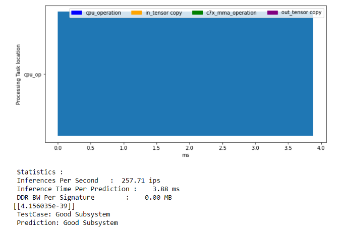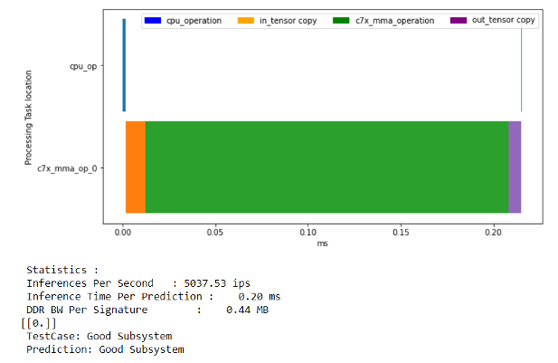You can now run both notebooks to run the inferences with and without deep learning acceleration. You can see more than 20x speed up due to the accelerator compared to running this CNN model just on the ARM processing cores. The model running on the ARM core is taking 3.88msec for one inference. On the other hand, deep learning acceleration enables the same inference in only 0.2 msec. ![MV CNN Model](./resources/6_5_inf_arm.png) ![MV CNN Model](./resources/6_5_inf_dl.png) <hr> ### Next Steps That's it! We have seen the complete flow of creating a model, compiling the model and deploying the edge inference on the edge AI starter kit EVM. The flow is exactly the same for any use case you may have for your application. ### References - Dau, Hoang Anh, Eamonn Keogh, Kaveh Kamgar Chin Chia Michael Yeh, Yan Zhu, Shaghayegh Gharghabi Chotirat Ann Ratanamahatana Yanping Chen, Bing Hu, Nurjahan Begum, Anthony Bagnall, Abdullah Mueen and Gustavo Batista “The UCR Time Series Classification Archive" https://www.cs.ucr.edu/~eamonn/time_series_data_2018/ - Z. Wang, W. Yan, T. Oates, "Time Series Classification from Scratch with Deep Neural Networks: A Strong Baseline", 2017 International joint conference on neural networks (IJCNN) Return to <a href="6_end_to_end_ai.html#6-1-live-video-analytics-with-usb-camera">< Part 6: End-to-end AI application development </a> <hr> <div align="center" style="margin-top: 4em; font-size: smaller;"> <a rel="license" href="https://creativecommons.org/licenses/by-nc-nd/4.0/"><img alt="Creative Commons License" style="border-width:0" src="../web_support/cc_license_icon.png" /></a> This work is licensed under a <a rel="license" href="https://creativecommons.org/licenses/by-nc-nd/4.0/">Creative Commons Attribution-NonCommercial-NoDerivatives 4.0 International License</a>.</div>