Introduction
This module provides an overview of the ultrasonic gas meter design and testing process. The gas meter design and test process involves a series of iterative tests that are conducted in an order designed to minimize the amount of time spent in evaluating transducers and new tube designs. While the estimated time to get to a working configuration is less than an hour, subsequent tests can require several weeks to complete. It is assumed that the reader already has a basic understanding of ultrasonic gas metering concepts.
Prerequisites
Hardware
Required Hardware for testing:
- The MSP430FR6043 EVM
- Ultrasonic flow tube
- 2x transducers
Software
Required software for testing:
- Ultrasonic Design Center GUI (requires Java)
Recommended Resources
This academy assumes the base knowledge from these resources is already familiar and understood:
- Ulrasonic Gas Meter Quick Start Guide: Overview to get up and running with TI's Ultrasonic Gas Metering Platform.
- Ultrasonic Gas Meter TI Design User's Guide: Detailed information about the theory and operation of the platform.
Gas Flow Measurement Overview
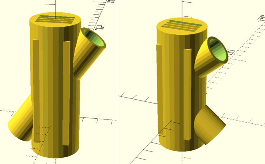
Transaxial and Reflective Tube Designs
Ultrasonic gas meters typically use two transducers which sequentially transmit an upstream and downstream signal through a pipe in which gas can flow. There are two predominant gas tube configurations found in the market: trans-axial(transducers face each other directly) and reflective(transducers face a reflecting surface).
Gas flow tubes are commonly used in residential and industrial gas meters. They are also commonly found in respirators and portable breathing machines.
Delta time of flight and flow measurement
There are two measurements(upstream and downstream) which must be taken in order to determine the upstream and downstream absolute time of flights. The time registered difference between these measurements is used to determine the delta time of flight. The delta time of flight, and two absolute time of flight measurements are used to determine the velocity as shown in the equation below.
Velocity = L/2 X deltaToF/(absToFUpStream)X(absToFDownStream)
Where L is the component of the ultrasonic path length which is parallel to the flow, deltaToF is the delta Time of Flight, and absToFUpstream and absToFDownstream are the upstream and downstream absolute Time of Flight respectively.
When gas flows through a tube, the upstream time of flight is increased while the downstream time of flight is decreased. The difference between the upstream and downstream time of flight(delta Time of Flight) increases based on the velocity of the gas flowing through the tube. This velocity is translated into volume flow rate by scaling the velocity by a meter constant which corresponds to the cross sectional area of the tube.
TI's Ultrasonic Gas Metering Solution
TI’s single chip solution comprises the majority of functionality required for gas metering applications as depicted in the figure below.
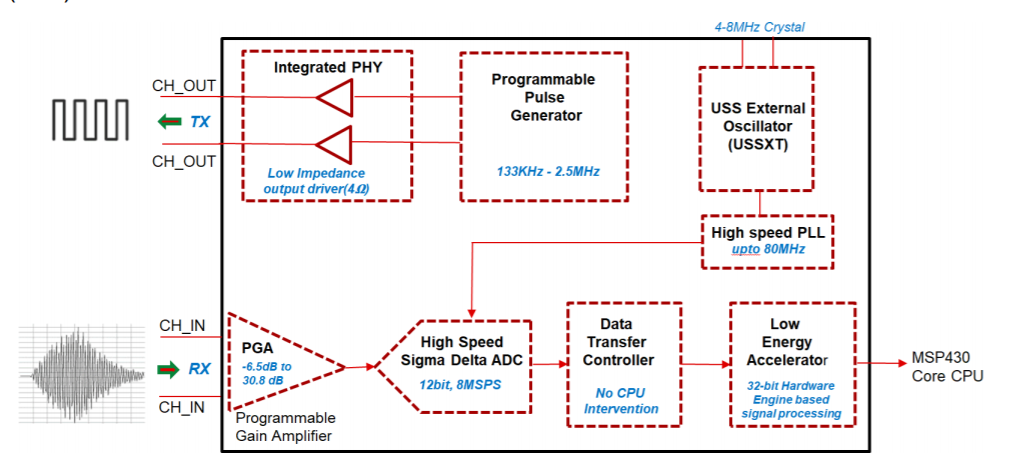
TI's ultrasonic sensing subsystem (see Figure above) comprises a programmable pulse generator (PPG) and a high-speed sigma delta analog to digital converter with a programmable gain amplifier (PGA) that can autonomously excite and capture ultrasonic waveforms for subsequent processing by the integrated Low Energy Accelerator(LEA). The LEA provides low power signal processing acceleration for common signal processing functions(correlation, filtering, interpolation, etc.).
This ultrasonic subsystem first excites the “upstream” transducer connected to CH0_OUT while capturing the waveform from a “downstream” transducer connected to CH0_IN. The ultrasonic subsystem subsequently excites the “downstream” transducer connected to CH1_OUT while capturing the waveform from the “upstream” transducer connected to CH1_IN. These waveforms are then processed by the LEA to determine the difference between the upstream and downstream time of flight.
TI’s ADC based correlation approach varies from commonly available TDC zero crossing approach in the way that the Absolute and Delta Time of Flights are determined. For the TDC zero crossing approach, a threshold is used with a timer to find the start of the signal with subsequent zero crossing detection.
TDC Based Zero Crossing Approach
This common approach determines the upstream and downstream absolute time of flight and subtracts them to determine the delta Time of Flight. Because there is a dependency on the amplitude of the signal (which will vary with different gas mixtures and flow conditions), this approach will typically give a higher standard deviation in measurements. This approach is depicted below.
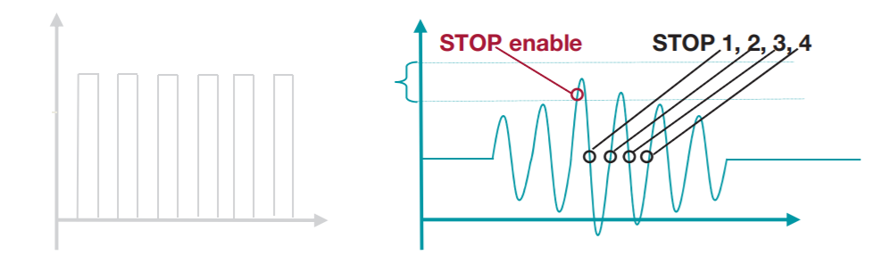
ADC Based Correlation Approach
An ADC Based Correlation approach for absolute time of flight implemented with TI’s solution is depicted in the figure below. In this approach, a frequency sweep binary pattern used to transmit the signal in both the upstream and downstream direction is first correlated with the received signal. The envelope of this correlated signal is then computed and the intersection between a specified threshold and that envelope is then calculated. This approach is depicted in the figure below.
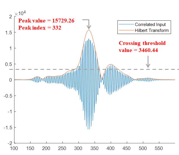
For determination of the delta Time of Flight, the results from the absolute time of flight calculations are used to predict the region over which the peak of the correlation between the upstream and downstream ADC captures should be determined. The upstream and downstream ADC captures are then correlated over this region with subsequent interpolation to determine the delta Time of Flight. Because this correlation acts like a low pass filter, the standard deviation in measurements is much smaller in this approach than can be found with other timer based (TDC) approaches.
Gas Meter Design Process
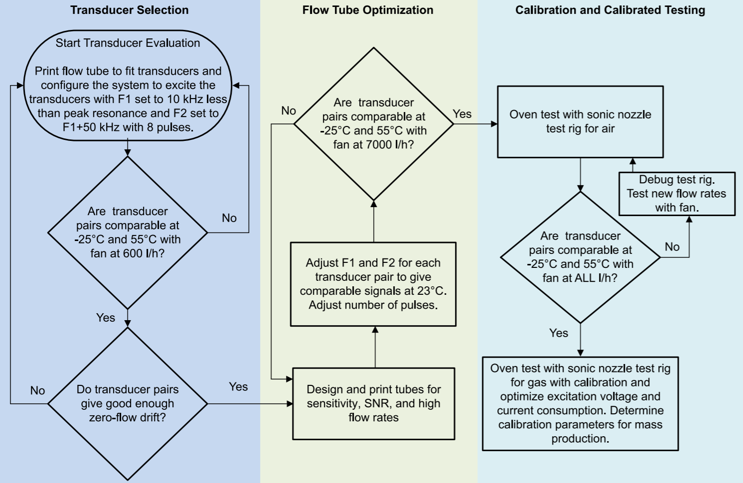
Because there are tradeoffs in tube design which can affect the robustness, repeatability, and sensitivity of the tube in testing, it’s important to repeat repeatability and standard deviation testing any time the tube design is changed. The overall gas meter design process is shown in the flow graph for -25C to 55C operation below. (some markets require -10C to 55C operation) Transducer pairs giving results which are within a few percentage points of each other are considered comparable.
Gas Flow Testing
When developing a gas meter, there are a series of tests, listed below, that should be conducted in air to ensure that the transducers and tube design will meet performance requirements before testing in methane. How to conduct these tests is described in detail in this section.
Transducer and Tube Tests:
Standard Deviation Testing: This test is conducted to confirm an initial configuration is working as anticipated with a standard deviation of 200-1000 picoseconds. The standard deviation can be further reduced by increasing the number of pulses used in repeatability testing.
Comparative Flow Testing: This test is conducted to confirm that there is sufficient repeatability across a representative number of transducer pairs to enable cost effective calibration for mass production. Error spreads between transducer pairs are expected to be within 6% over operating temperatures at low flows and within 3% over operating temperatures at higher flows.
Zero Flow Drift Testing: This test is conducted to confirm that the zero flow drift of a representative number of transducer pairs will meet the requirement for minimum detectable flow. Zero flow drift results between 200-500 picoseconds across multiple transducer pairs are expected.
Repeatability Flow Testing: This test is conducted to confirm that the tube design is robust at high flow rates and to provide a baseline for comparative debug at lower flow rates before migrating to a calibrated flow testing. Repeated flow test results are expected to be within 0.5% of each other at both high and low flow rates. Repeatability tests should be repeated with calibrated air and methane test rigs to debug issues which may be specific to these test environments.
Calibrated Flow Testing: This test is conducted to confirm that a representative number of gas meters will meet certification requirements. Calibrated air flow tests are expected to give results comparable to the results previously found in repeatability testing over operating temperature extremes. Subsequent tests with various gas mixtures are expected to provide results which can meet certification requirements by calibrating individual meters in air at room temperature.
Which test is critical for cost effective mass production?
Initial Configuration
This section describes the process by which users can quickly get to a working configuration with TI's ultrasonic gas meter solution. Standard deviation results will vary based on the sensitivity of transducers used and the ultrasonic path of a given tube.
The figures below depict the basic and advanced configuration parameters where each configuration parameter is described below:
NOTE:
When powering the board from USB, noise from the laptop power supply can often times be reduced by disconnecting power from the laptop.
Basic Configuration Parameters
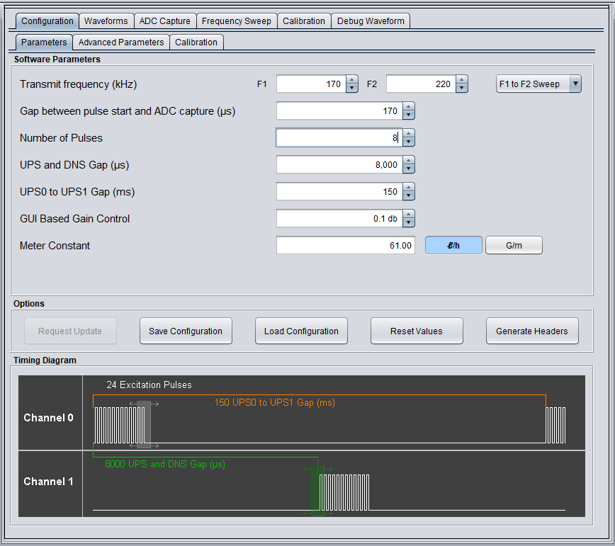
F1: Start Transmit Frequency – the start frequency for excitation of both the upstream and downstream transducer.
F2: End Transmit Frequency – the end frequency for excitation of both the upstream and downstream transducer.
Gap Between pulse start and ADC Capture: The start time for the ADC capture.
Number of Pulses: The number of transmit pulses used to excite the upstream and downstream transducers – this should be set to 8 for an initial configuration. Eight pulses is the minimum number of pulses in which a significant amount of frequency information can be encoded.
UPS and DNS Gap: The time between Upstream(UPS) and Downstream(DNS) measurements. Further detail on this parameter is provided in the next section.
UPS0 to UPS1 Gap: The time between flow measurements. This is typically set to 1000 or 2000 seconds for field operation. When conducting standard deviation experiments, it should be set to 150ms to minimize the required test time.
GUI Based Gain Control: Programmable gain of the Upstream and Downstream captured signals. This should be set to a value that gives between 800 and 1000 counts in the ADC capture.
Meter Constant: This is a flow rate scaling constant. This should be determined with a reference meter in series in preparation for Calibrated Flow Testing.
Request Update: Sends the configuration to the connected platform.
Advanced Configuration Parameters
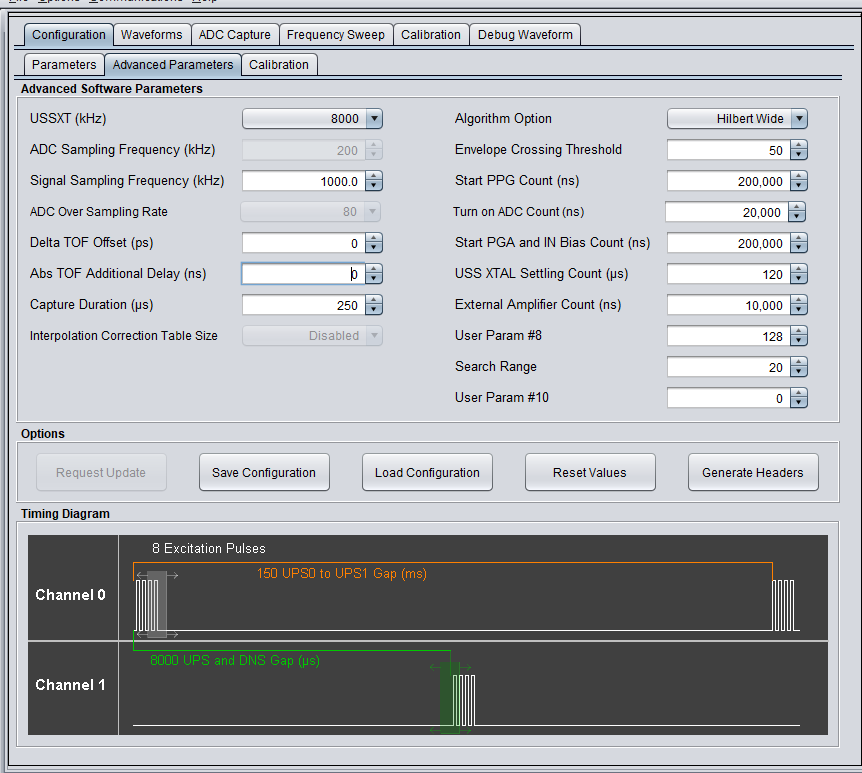
Signal Sampling Frequency: This should be set to 1000 for 200kHz transducers and 2000 for 500kHz transducers.
Capture Duration: Set to 250us. This parameter is memory constrained to 250us with a signal sampling frequency of 2000(500kHz transducers). Although it can be increased to 400us when a signal sampling frequency of 1000(200kHz transducers) is used, a 250us sampling window should suffice for initial testing.
USS XTAL Settling Count: Set to 120us when resonator is used and 4000us when a crystal is used.
User Param #8: Set to 128. This parameter determines whether additional custom pulses will be used after the initial transmit pattern. A setting of 384 enables additional custom pulses while a setting of 128 disables them. Additional pulses are used to reduce the residual energy emitting from a transducer after excitation. An alternative way of doing this is to continue exciting the transducer at a frequency which is beyond its excitation band. Reducing this energy is discussed in the context of calibrated flow testing in methane because the increased speed of sound in methane will reduce the time between excitation and ADC capture.
Search Range: Set to 20. This parameter determines how many samples to search over for the peak of the envelope in the absolute time of flight calculation based on the previously determined location of the peak. Once the gas meter has undergone all other testing, this value may be experimentally reduced under anticipated pulsating flow conditions to reduce power consumption.
Determining the ADC Start Capture Time
The ADC start capture time can be roughly determined with the following equation:
ADC Start Capture Time = (Ultrasonic Path Length/Speed of Sound) – 40us
As an example, for 7cm spacing between two transducers:
ADC Start Capture Time = 0.07/343 -125 = 204 us – 40us = 164us (The ADC Start Capture Time MUST be an EVEN number!)
Set F1 to 170 and F2 to 172 for 200kHz Transducers. Set F1 to 470 and F2 to 472 for 500kHz Transducers.
Capture the signal and adjust ADC Start Capture Time to center the signal in the capture window.
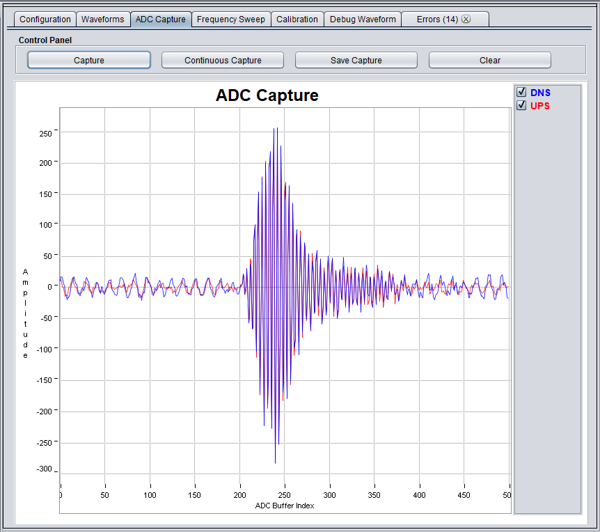
Adjust GUI gain to get around 250 ADC counts. The figure below depicts an expected ADC capture.
ADC Capture of Centered Signal:
Determining F1 and F2 Transmit Frequencies
Set F1 to 170 and F2 to 172 for 200kHz Transducers. Set F1 to 440 and F2 to 442 for 500kHz Transducers.
Set number of captures to 30 with step size of 3 for Frequency Sweep.
Select Frequency Sweep. The figure below depicts a typical frequency sweep.
Frequency Sweep:
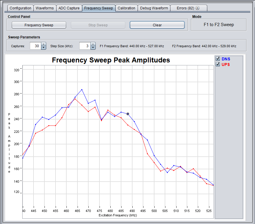
F1 should be set to the Peak Frequency – 10 kHz while F2 should be set to F1 + 50kHz
For the frequency sweep in the figure above:
F1 = 465 - 10 = 455 F2 = F1+50 = 505
After setting F1 and F2 and requesting an updated, adjust the GUI Gain to get around 800 ADC Counts. (This is to ensure that the results aren't saturated when operating at lower temperatures.)
Standard Deviation Testing
Standard deviation testing ensures you have a working initial configuration which is providing anticipated results. Standard deviation results can be improved by increasing the number of pulses used in the configuration.
Std Dev Test Process
Put the tube with transducers in a metal can with a hole for transducer wires. Connect the EVM ground to the can. Move the S5 switch to the EXT position. Connect external 3.3V power supply to TP1(AFE 3V3) and TP2(GND). Select the Start Button in the Waveforms tab to begin Waveform Capture. The standard deviation of the delta ToF waveforms should be between 200ps and 1000ps after 30 seconds of capture as depicted in the figure below.
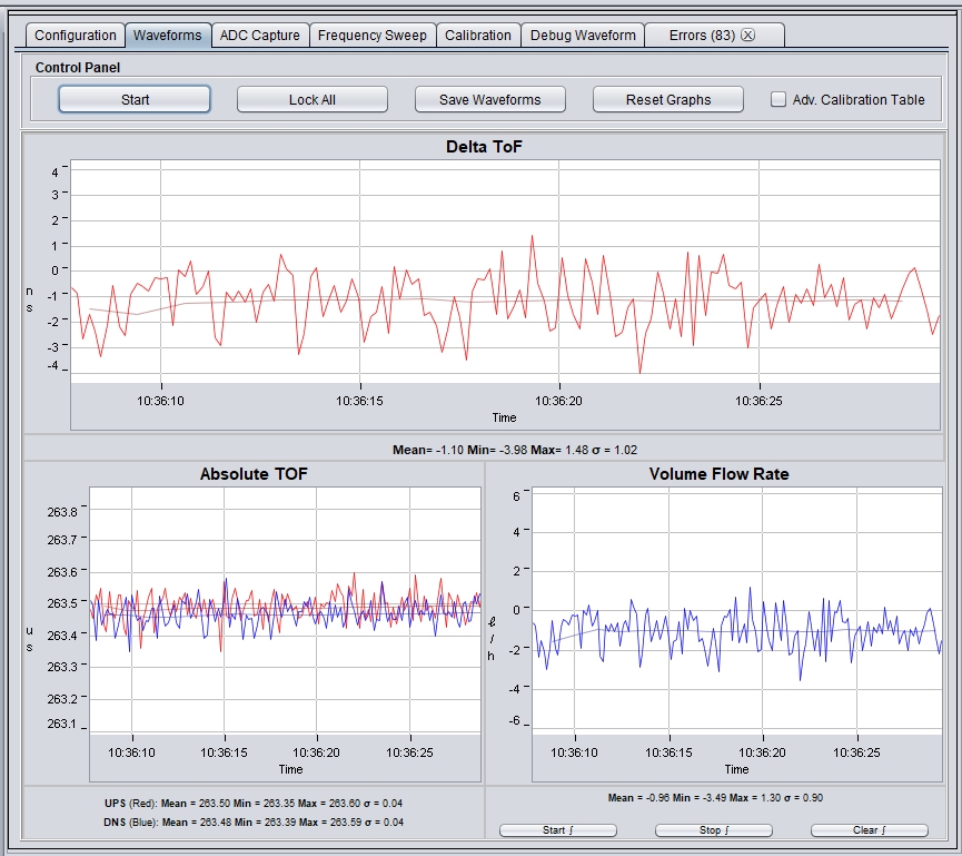
One of the factors that can have a significant impact on the standard deviation is the number of transmit pulses used. Although increasing the number of transmit pulses can reduce the standard deviation and the number of measurements required to get an accurate reading, it can have a negative effect on repeatability. We’ll revisit this topic in the context of repeatability and tube optimization.
Which parameter can be adjusted to decrease the standard deviation?
Comparative Flow Testing
Comparative flow testing ensures that variations in transducer pair frequency response can be cost effectively calibrated for mass production. It is therefore critical to conduct this testing early on in the design process to avoid wasting time with transducers that can’t meet requirements. Although it's anticipated that there will be some variation in the ultrasonic path of different tubes, the ratio of reported flows between two tubes over temperature is expected to be close enough to enable calibration of production gas meters at room temperature. Comparative flow testing requires a climatic chamber, two flow tubes(with transducers), two MSP4306043 Platforms(and PCs), a brushless DC fan, and a power supply. The amount of time required to compare two transducer pairs over three temperature settings can be 8 hours for climatic chambers requiring 3 or 4 hours to fully stabilize at a given temperature.
CF Setup
NOTE:
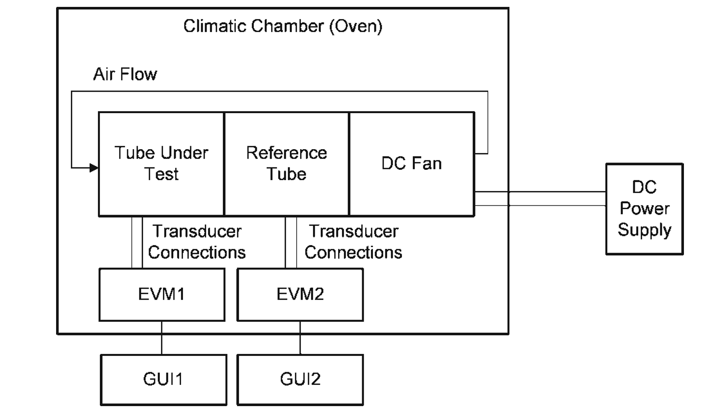
A brushless DC fan which is capable of operating at low voltages and flow rates such as the Micronel D301L-012GK-2 should be used in this test setup.
Connect two tubes to two different EVMs. Connect a fan to both tubes so that air is pulled through both tubes and recirculated within an oven. Each EVM should be connected to a separate computer with a GUI and the configuration determined by the initial configuration process. The crystal should be populated and used on both EVMs. The figure below depicts the test setup.
Comparative Flow Testing Setup:
CF Process
The process for comparative flow testing involves comparing the ratio of reported flow results between two transducer pairs at 23C, 55C, and -10C. This process is repeated over at least 10 transducer pairs as depicted in the figure below.
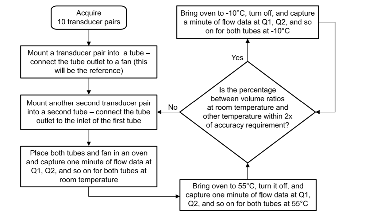
After two tubes have been setup as shown in the previous section, adjust the voltage of the fan to give ~60ns of dToF(Q1) with the oven off and the oven door closed at room temperature. Reset the graphs at the same time and capture and save one minute of waveforms and means for both tubes.
Adjust the voltage of the fan to give ~400ns of dToF(Q2) with the oven off and oven door closed at room temperature. Reset the graphs at the same time and capture and save one minute of waveforms and means for both tubes.
Turn on the oven and set the oven temperature to 55C. Let the oven stabilize at 55C for a few hours with the fan running.
Turn off the oven, reset graphs, capture and save one minute of waveforms and means.
Reduce the fan voltage to the setting previously used to give ~60 ns of dToF(Q1). Reset the graphs at the same time and capture and save one minute of waveforms and means. Bring oven to -10C and let stabilize with fan on for a few hours.
Turn off oven, reset graphs, capture and save one minute of waveforms and means. Increase fan voltage to setting previously used to give ~400 ns dToF, reset graphs at the same time, capture and save one minute of waveforms and means.
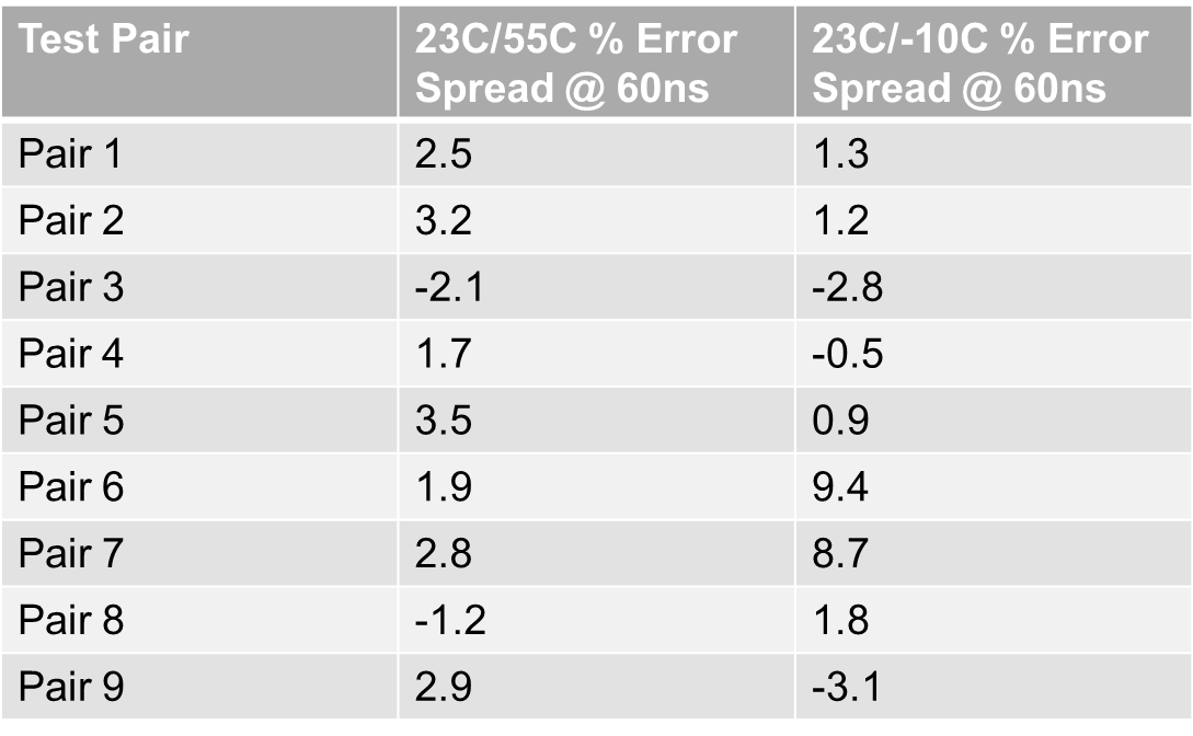
Calculate the reference and test tube % Ratio and % Error Spread between 23C and 55C at 60ns dToF using the following equations:
% Ratio = 100*(1-(Mean@23C/Mean@55C))
% Error Spread = % Reference Ratio - % Test Ratio
Calculate the reference and test tube % Ratio and % Error Spread between 23C and -10C at 60ns dToF by replacing the Mean@55C with the Mean@-10C in the equations above.
Repeat these calculations for 400ns dToF data.
Replace the transducers in the test tube with another pair of transducers and repeat the same tests and calculations. For each pair of transducers, you should be able to plot the spread in % Errors against the reference pair as depicted below.
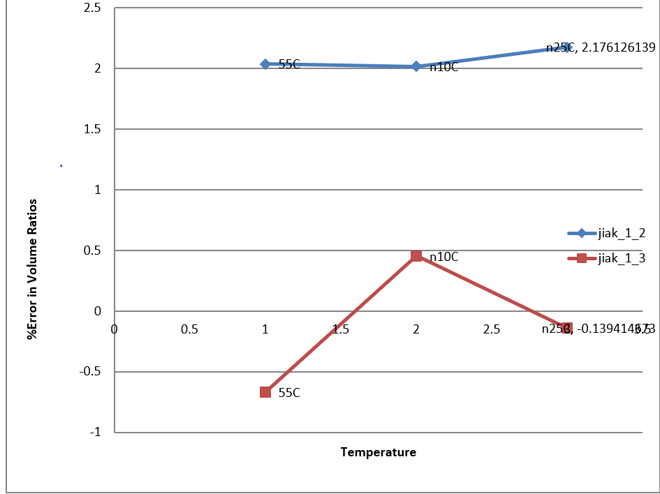
CF Analysis
Outliers with error spreads exceeding target requirements(for example: 6% Error spread) should be retested. If the percentage of transducers exceeding requirements is small enough(after repeat testing), screening transducers at two temperature points may be possible. Increased consistency across transducer pairs may also be achieved with a transducer that has less shift in frequency response over temperature and is more dampened. The diagram below depicts two outliers with 9.8% and 8.7% spread which were due to ambient noise during initial testing. This noise was subsequently mitigated by conducting tests at times when neighboring machines weren't in operation.
Spread in Errors Across 10 Transducer Pairs:
Why should comparative flow testing be conducted as soon as you have a working configuration?
Zero Flow Drift Testing
Zero flow drift testing determines the variation in the delta Time of Flight that occurs over the range of operating temperatures. This test is important in determining the minimal detectable flow of a gas meter over its operating temperature range. It’s also important in order to identify any strange behavior in the absolute time of flight early on. Zero flow drift tests require 12 hours to ensure the oven temperature is fully stabilized over 4 operating temperatures. If the climatic chamber is large enough, multiple platforms and tubes can be tested simultaneously.
NOTE:
The temperature range over which zero flow testing should be conducted will vary based on the target market requirements.
ZFD Setup
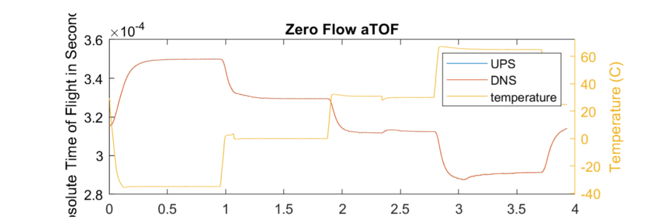
The tube should have both ends sealed and be put into a grounded can with a hole for the transducer wires in the same way testing is conducted for standard deviation. This can should be placed in the oven along with the EVM and waveform data should be collected while the oven cycles from -25C to 55C in a series of steps over several hours. The figure below depicts the absolute time of flight as a function of logged data from -35C to 65C (some markets require testing over a larger range).
Zero Flow aToF over Temperature:
The corresponding zero flow drift in the delta Time of Flight is depicted in the figure below.
Zero Flow dToF over Temperature:
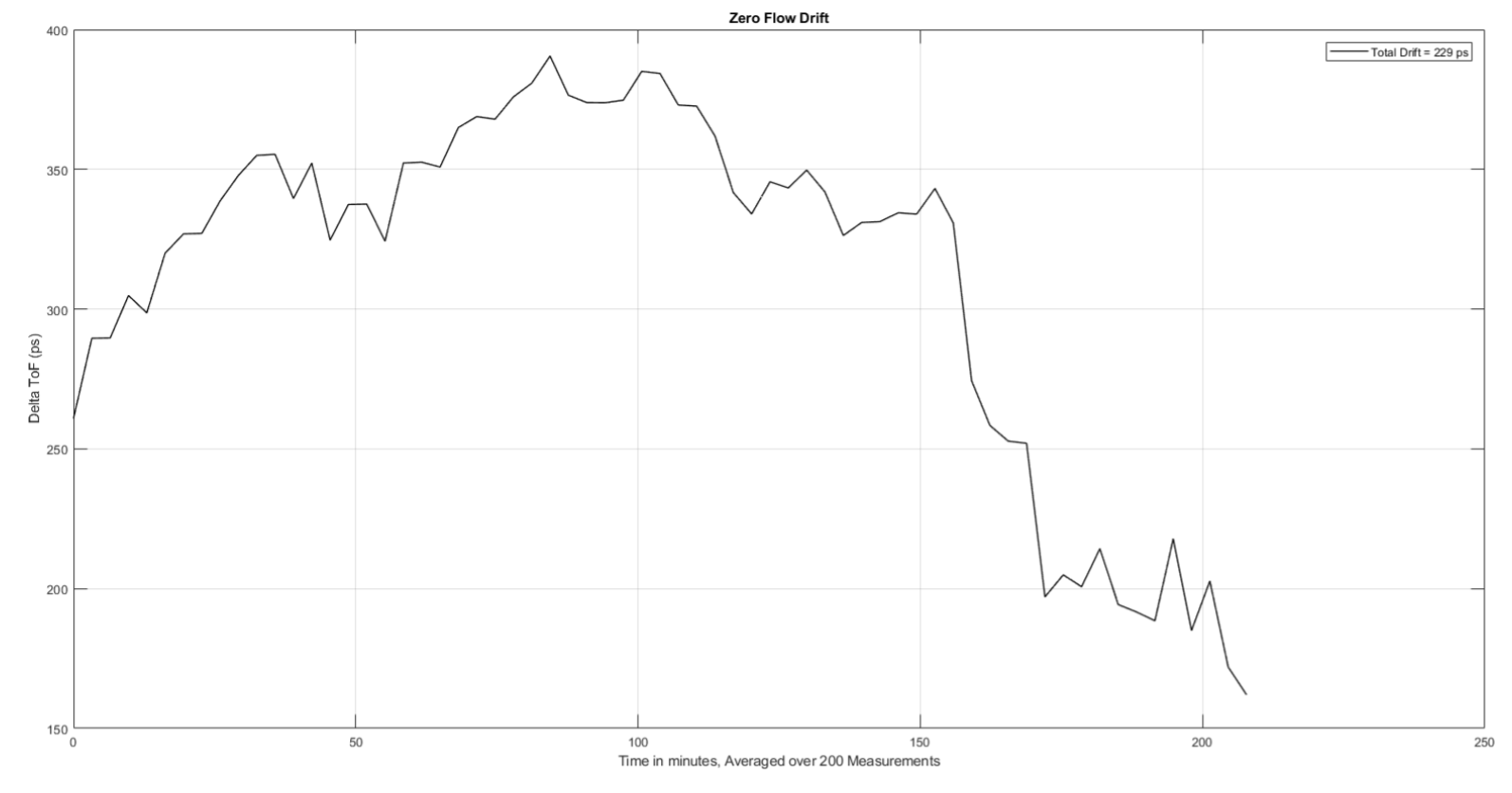
ZFD Analysis
Because the zero flow drift can improve with impedance matched transducers, it’s important to test a representative set of transducer pairs randomly selected from a production lot (at least 10). Variations in zero flow drift across transducer pairs should be statistically understood when determining the minimum detectable flow of meters in mass production.
Repeatability Testing
Repeatability testing ensures that there aren't any transient noise issues which might be polluting measurement results. Repeated measurements are expected to give measurement results which are within 0.5% of each other when testing with the same fan and tube at a given operating temperature. Repeatability testing should first be conducted with a fan over low, medium, and high flow rates at room and extreme operating temperatures.
Repeatability Test Setup
The same test setup used for comparative flow testing can be used for repeatability testing of two tubes at the same time. Repeatability tests should also be conducted with a calibrated flow test setup to enable comparative debug of issues which might be introduced by the test rig. It's important to note that the transducers should not be removed/replaced between repeatability tests as small changes in the physical distance between transducers can affect repeatability results.
NOTE:
Repeatability testing should also be conducted with the calibrated test setup.
Repeatability Analysis
At high flow rates, there may be variations in the amplitude of the downstream received signal. This can cause significant variations in the absolute Time of Flight measurements. Because the absolute Time of Flight measurements are used to determine which correlation peak to lock onto for the delta Time of Flight measurement, variations in the absolute Time of Flight greater than half a cycle can cause cycle slips in the measurement results. The figures below depict the ADC capture and corresponding cycle slip in the waveforms.
Asymmetry in Upstream/Downstream ADC captures:
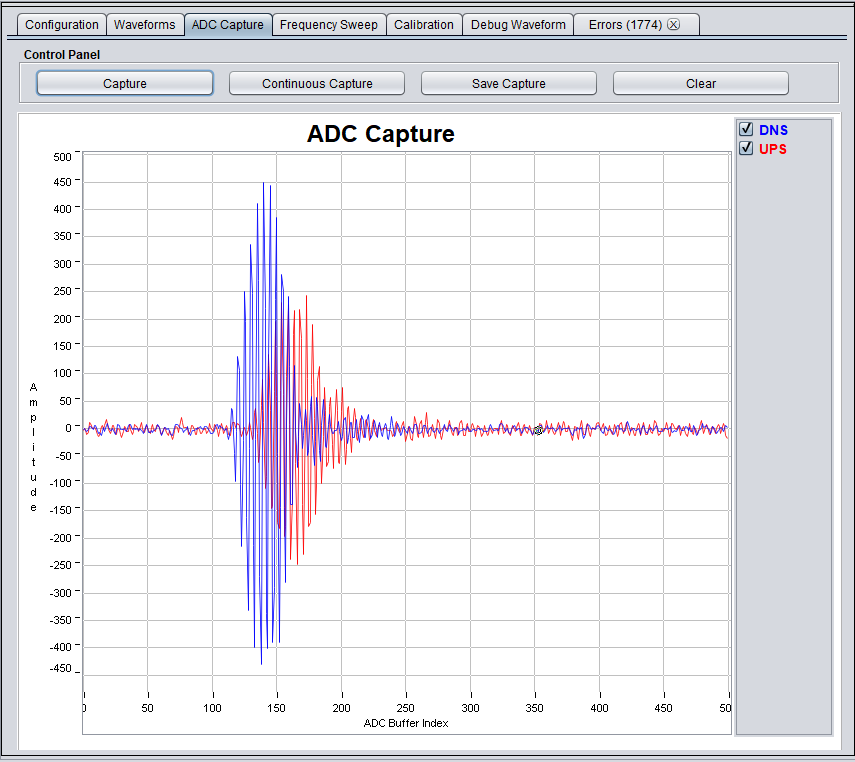
Cycle Slips in Waveform Data:
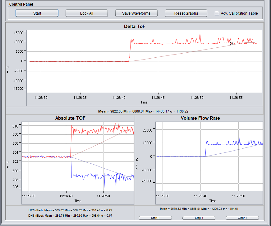
Cycle slips might also occur at higher flow rates at -25C due to changes in the ADC capture which cause the absolute time of flight measurement to shift by more than half a cycle. Using more dampened lower frequency transducers or modifying the tube design to reduce the velocity of the flow in the tube can resolve these problems. If the shift in absolute time of flight is due to continued excitation of the transducer at these colder temperatures, the F2 transmit frequency can also be increased to more quickly dampen the excitation.
When capturing repeatability data, independent trials should be repeated at least 3 times at target flow rates. The variations in reported measurement results should then be determined to identify potential issues with the tube design or the test environment. The table below depicts 3 repeated flow rate measurement means for four different flow rates conducted at room temperature. From this table it can be seen that the percent variations in test results is much higher at lower flow rates. Each mean was based on 300 measurements in this case.
Repeat Measurements:
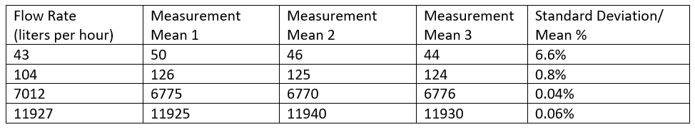
The standard deviation of results can be improved by capturing more samples if the noise is Gaussian. The accuracy of the measurements should increase based on the square root of the number of samples taken so in order to cut the standard deviation in half, four times as many samples should be used to calculate the mean. In the event that the noise isn’t Gaussian, the noise source must be identified and controlled.
Repeatability testing should also be conducted at representative low, medium and high flow rates at operating temperature extremes (-25C and 55C).
Enough experiments should be conducted to determine the statistical probablility that meters will meet specification limits in mass production. This is typically calculated with a Cpk metric. The formula for the calculation of Cpk is Cpk = min(USL - μ, μ - LSL) / (3σ) where USL and LSL are the upper and lower specification limits, respectively. A process with a Cpk of 2.0 is considered excellent, while one with a Cpk of 1.33 is considered adequate.
Why is it important to zero flow drift test multiple transducer pairs?
Calibrated Air Flow Testing
Calibrated air flow testing typically involves a sonic nozzle test setup. The velocity of a gas flowing through a sonic nozzle is a function of the diameter, the temperature, and the pressure of the gas flowing through it as depicted in the figure below. These nozzles are also known as de Laval nozzles and are commonly used in rockets.
NOTE:
This is a simplified test setup which is specific to air. Testing should be conducted with a mixed gas test setup after satisfactory results have been achieved with air.
Sonic Nozzle Temperature and Pressure:
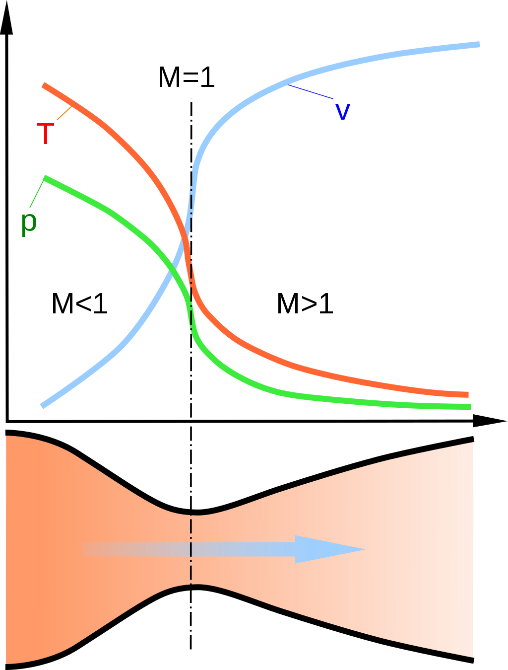
In order to accurately determine the flow through a combination of sonic nozzles, the pressure and temperature of the gas (on both sides of the nozzle) must be known along with the diameter of the nozzle(and the gas composition). An array of nozzles is typically actuated in order to achieve a calibrated flow rate.
Test Setup
The figure below depicts a sonic nozzle test setup used for calibrated air flow testing.
Sonic Nozzle Test Setup:
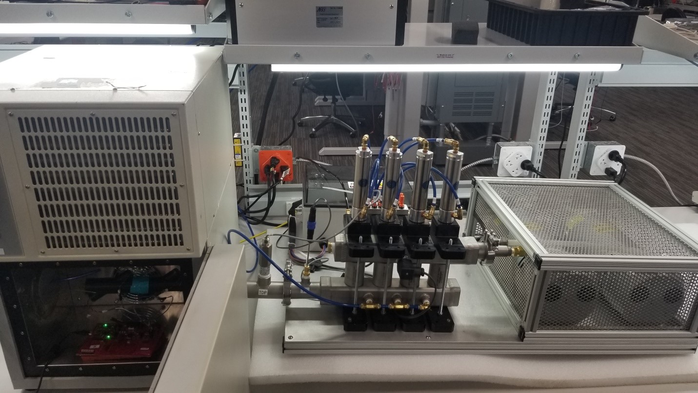
At the far right are two vacuum pumps which pull air through an array of four sonic nozzles with different diameters. A Unit Under Test(UUT) is connected to the inlet of the system inside of climatic chamber. There is a dedicated controller that actuates the sonic nozzles and determines the calibrated flow rate based on multiple pressure and temperature sensors connected throughout the system. The PC interface to this test system is depicted in the figure below.
Sonic Nozzle GUI:
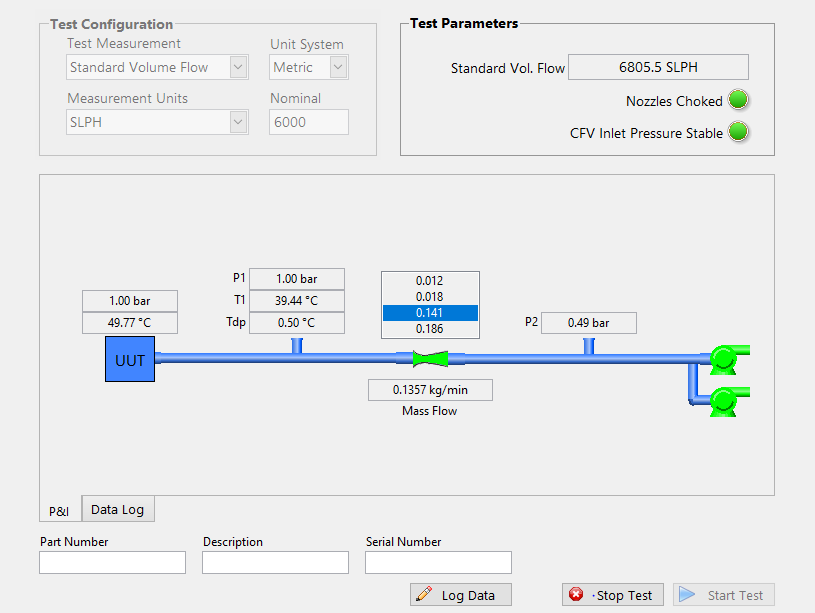
In this configuration, although a 6000lh configuration is specified, the closest flow rate the system could provide was around 6805lh. The 0.141 inch diameter sonic nozzle was actuated in order to achieve this flow. For flow rates around 12000lh, the 0.186 inch diameter would be actuated. For flow rates around 18000lh, both the 0.141 and 0.186 nozzles would be actuated.
Analysis
After completing repeatability testing with a fan, repeatability testing with the sonic nozzle test system should be repeated at low flow rates. Because a sonic nozzle test system pulls(rather than recirculates) air in the climatic chamber, a heat exchanger with compressed dry air should be used in the climatic chamber to ensure that the air being pulled through will be at a stable temperature before reaching the UUT.
Unlike diaphragm(mechanical) meters, ultrasonic gas tubes don’t restrict the flow of gas. As a result, they are susceptible to small changes in air flow when there are changes in the ambient pressure due to air conditioner cycling or door openings. It’s important to capture several hours of waveforms at low flow rate to determine the frequency of these events and their potential effects on results. The figure below depicts some low frequency noise which are commonly due to ambient changes in air pressure. Nearby vents and doors should remain closed to mitigate these effects during testing.
Sonic Nozzle Waveforms:
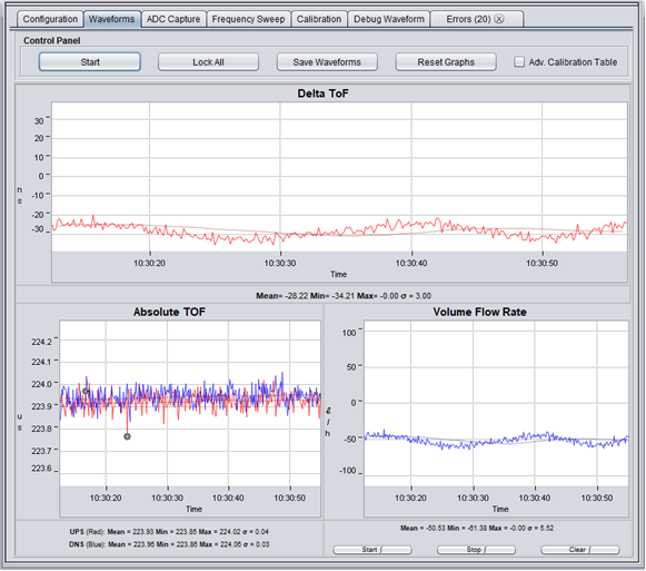
Capturing waveforms when the AC isn’t used or when others aren’t present in the lab operating other machines can give good insights into what might be causing noise to show up at lower flow rates.
How can noise issues in sonic nozzle testing be debugged?
This work is licensed under a Creative Commons Attribution-NonCommercial-NoDerivatives 4.0 International License.