Introduction

This module provides an overview of the ultrasonic water flow meter design and testing process.

Ultrasonic sensing uses the time of flight (TOF) of an ultrasonic wave within any liquid or gas medium and its dependency on the flow rate to measure and calculate volume flow. This technique uses the difference in the propagation time of the ultrasonic wave when transmitted into and against the direction of the flow. This technology is robust and accurate in measuring volume flow rates across a wide dynamic range.

The water flow meter design and test process involves a series of iterative tests that are conducted in an order designed to minimize the amount of time spent in evaluating the performance of the meter, calibration and repeatability for production. While the estimated time to get to a working configuration is less than an hour, subsequent tests can require several weeks to complete. It is assumed that the reader already has a basic understanding of ultrasonic water flow metering concepts.

Prerequisites

Hardware

Required Hardware for testing:

• MSP430FR6043 EVM
  • For additional integrated memory: MSP430FR6047 EVM
  • For lower cost and performance, pin compatible devices: MSP430FR6005 / MSP43FR6007
• Ultrasonic water flow tube with 2x (pair) transducers

Software

Required software for testing:

• Ultrasonic Design Center GUI (requires Java(JRE 1.7))

Recommended Resources

This academy assumes the user has a basic knowledge based on these resources:

• Ulrasonic Water Flow Meter Quick Start Guide (Rev B): Overview to get up and running with TI's Ultrasonic Water Flow Metering Solution.
• Ultrasonic Water Flow Meter TI Design User's Guide: Detailed information about the theory and operation of the platform.
• Waveform capture based ultrasonic sensing water flow metering technology: Describes the time-of-flight (TOF) approach for water flow measurement using ultrasonic sensing (USS) technology.
• USS Water Flow Rate Calibration: Calibration methodology for flow rate and temperature variation.
• Additional Ultrasonic Applications Overview: Overview of additional ultrasonic liquid and gas applications.

Water Flow Measurement Overview

Transaxial and Reflective Tube Designs

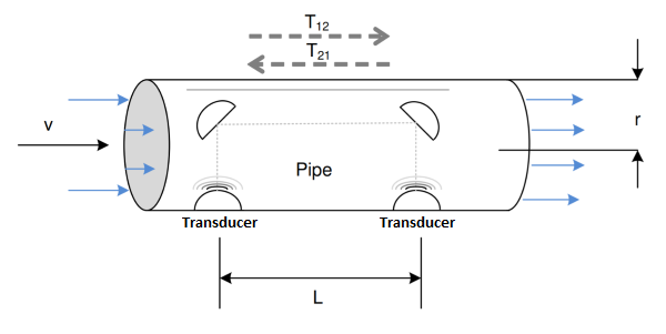
Ultrasonic water flow meters typically use two transducers which sequentially transmit an upstream and downstream signal through a pipe in which water can flow. There are two predominant water flow tube configurations found in the market:

Trans-axial: The transducers face each other directly.

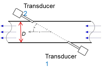
Reflective: The transducers face a reflecting surface.

Water flow tubes are commonly used in residential and industrial water flow meters.

Delta time of flight and flow measurement

There are two measurements, upstream and downstream, which must be taken in order to determine the upstream and downstream absolute time of flights. The time registered difference between these measurements is used to determine the delta time of flight. The delta time of flight, and two absolute time of flight measurements are used to determine the velocity as shown in the equation below.

Velocity = L/2 X deltaToF/(absToFUpStream)X(absToFDownStream)

Where L is the component of the ultrasonic path length which is parallel to the flow, deltaToF is the delta Time of Flight, and absToFUpstream and absToFDownstream are the upstream and downstream absolute Time of Flight respectively.

When water flows through a pipe, the upstream time of flight is increased while the downstream time of flight is decreased.
The difference between the upstream and downstream time of flight, called the delta Time of Flight, increases based on the velocity of the water flowing through the pipe. This velocity is translated into volume flow rate by scaling the velocity by a meter constant which corresponds to the cross sectional area of the pipe.

TI's Ultrasonic Water flow Metering Solution

TI’s single chip solution comprises the majority of functionality required for water flow metering applications as depicted in the figure below.

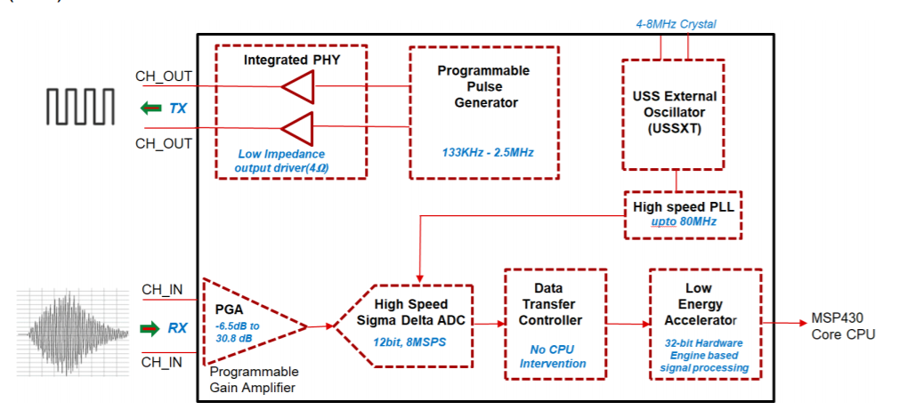
TI's ultrasonic sensing subsystem, as shown in Figure above, comprises of a programmable pulse generator (PPG) and a high-speed sigma delta analog to digital converter (ADC) with a programmable gain amplifier (PGA) that can autonomously excite and capture ultrasonic waveforms for subsequent processing by the MSP430 CPU and and integrated Low Energy Accelerator (LEA). The LEA provides low power signal processing acceleration for common signal processing functions like correlation, filtering, interpolation, etc.

This ultrasonic subsystem first excites the “upstream” transducer connected to CH0_OUT while capturing the waveform from a “downstream” transducer connected to CH0_IN. The ultrasonic subsystem subsequently excites the “downstream” transducer connected to CH1_OUT while capturing the waveform from the “upstream” transducer connected to CH1_IN. These waveforms are then processed by the MSP430 CPU with support from LEA to determine the difference between the upstream and downstream time of flight.

TI’s ADC based correlation approach varies from commonly available TDC zero crossing approach in the way that the Absolute and Delta Time of Flights are determined. For the TDC zero crossing approach, a threshold is used with a timer to find the start of the signal with subsequent zero crossing detection.

TDC Based Zero Crossing Approach

This common approach determines the upstream and downstream absolute time of flight and subtracts them to determine the delta Time of Flight.

Because there is a dependency on the amplitude of the signal, which varies with different water flow conditions, this approach will typically give a higher standard deviation in measurements. This approach is depicted below.

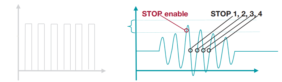
ADC Based Correlation Approach

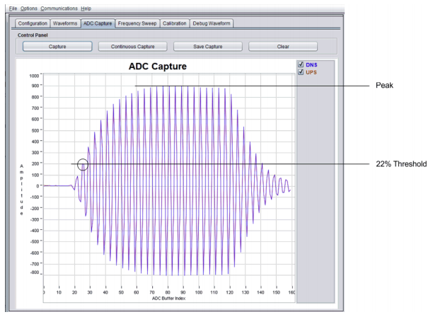
An ADC Based Correlation approach for absolute time of flight implemented with TI’s solution is depicted in the figure below.

In this approach, the peaks of each of the lobes of the received signal are computed and the intersection between a specified threshold and the maximum of the lobe peaks is then calculated. This approach is depicted in the figure below.

For determination of the delta Time of Flight, the results from the absolute time of flight calculations are used to predict the region over which the peak of the correlation between the upstream and downstream ADC captures should be determined. The upstream and downstream ADC captures are then correlated over this region with subsequent interpolation to determine the delta Time of Flight. Because this correlation acts like a low pass filter, the standard deviation in measurements is much smaller in this approach than can be found with other timer based approaches like TDC.

Water Flow Meter Design Process

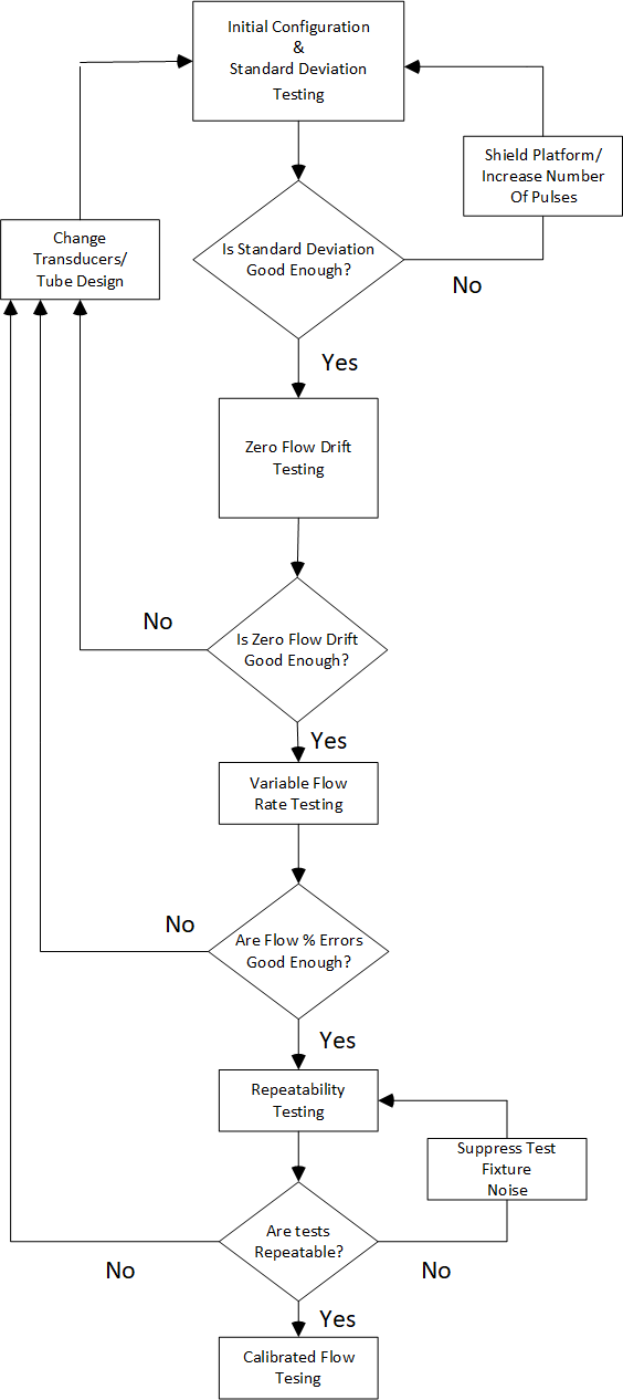
Some of the key aspects that are part of the water meter specifications is (a) the ratio of the highest flow rate supported (M4) and the lowest flow rate supported (M1) where the accuracy targets are met. This ratio of M4/M1 is the R value of the meter. The ability to achieve a high R or a very low M1 depends on the drift of the delta Time of Flight over temperature at zero flow or at those low flows. The flow of water through the pipe also has different characteristics depending on the pipe design depending on the flow rate and temperature that can impact the accuracy of the measured flow rate. Calibration is needed for a specific pipe design over the supported flow rate and temperature range. The overall design and test process is depicted in the flow chart below.

Water Flow Testing

When developing a water flow meter there are a series of tests that should be conducted to ensure that the transducers and pipe design can meet performance requirements. These tests are described in this section.

Initial Configuration

This section describes the process by which users can quickly get to a working configuration with TI's ultrasonic water flow meter solution. Standard deviation results will vary based on the sensitivity of transducers used and the ultrasonic path of a given tube. Because the Tx and Rx impedance are matched, it's unnecessary to change any of the discrete components when evaluating transducers with different impedance characteristics.

The figures below depict the basic and advanced configuration parameters where each configuration parameter is described below:

Basic Configuration Parameters

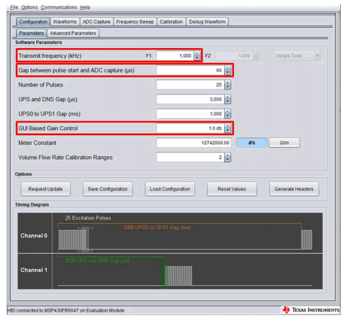
The F1, Gap, and Gain parameters are the only parameters which should be initially adjusted. All other parameters should be set to their default values for 1-MHz transducers. These parameters control the excitation, amplification, and ADC capture time between the ultrasonic transducers connected to the platform.

F1: Transmit Frequency – the nominal frequency of excitation of both the upstream and downstream transducers.

Gap Between pulse start and ADC Capture: The start time for the ADC capture, based on the anticipated ultrasonic time of flight between the two transducers.

Number of Pulses: The number of transmit pulses used to excite the upstream and downstream transducers – this should be set to 20 for an initial configuration.

UPS and DNS Gap: The time between Upstream(UPS) and Downstream(DNS) measurements. Further detail on this parameter is provided in the next section.

UPS0 to UPS1 Gap: The time between flow measurements. This is typically set to 1000 milli-seconds for field operation. When conducting standard deviation experiments, it should be set to 250ms to minimize the required test time.

GUI Based Gain Control: Programmable gain of the Upstream and Downstream captured signals. This should be set to a value that gives between 800 and 900 counts in the ADC capture. The input to the PGA is biased at 750mV with a max peak to peak input of 1000mV. The reference voltage for the Analog to Digital converter is generated internally.

Meter Constant: This is a flow rate scaling constant. This should be determined with a reference meter in series in preparation for Calibrated Flow Testing.

Request Update: Sends the configuration to the connected platform.

Advanced Configuration Parameters

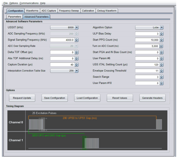
Signal Sampling Frequency: This should be set to 3.6 MHz for 1-MHz transducers and 7.2MHz for 2-MHz transducers.

Capture Duration: Set to 40us. This parameter needs to be increased for configurations with a larger number of pulses. We need to ensure the signal is fully captured with enough margin for shifts over the intended operating temperature range

USS XTAL Settling Count: Set to 120us when resonator is used and 4000us when a crystal is used.

Envelope Crossing Threshold: This determines which lobe the AbsToF algorithm will lock onto. Set this threshold to lock onto the earliest lobe peak that is above the noise. In the example shown in a later section, this lobe peak corresponds to a threshold of approximately 22%.

Search Range: This should be ignored. This is specific to gas algorithms and is not currently used by the water flow meter algorithm.

Determining the ADC Start Capture Time

The ADC start capture time can be roughly determined with the following equation:

ADC Start Capture Time = (Ultrasonic Path Length/Speed of Sound) – 10us

As an example, for 10 cm spacing between two transducers:

ADC Start Capture Time = 0.10/1480 = 67 us – 10 us = 57 us

Set F1 to 1000 for 1 MHz Transducers. Set F1 to 2000 for 2 MHz Transducers.

Capture the signal and adjust ADC Start Capture Time to center the signal in the capture window.

Adjust GUI gain to get around +/- 900 ADC counts. The figure below depicts an expected ADC capture.

ADC Capture of Centered Signal:

Determining F1, the Excitation Frequency

Set F1 to 800 for 1 MHz Transducers. Set F1 to 1600 for 2 MHz Transducers.

Set number of captures to 35 with step size of 12 for Frequency Sweep.

Select Frequency Sweep. The figure below depicts a typical frequency sweep.

Frequency Sweep:

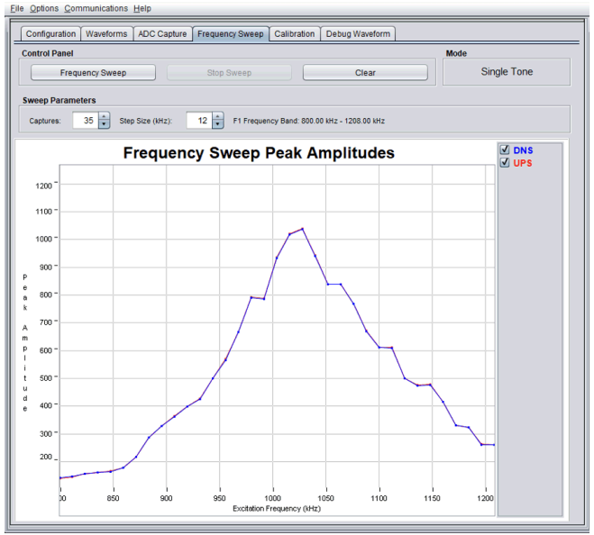
F1 should be set to the Peak Frequency.

For the frequency sweep in the figure above:

F1 = 1040

After setting F1 and requesting an update, adjust the GUI Gain to get around +/- 800 ADC Counts.

Standard Deviation Testing

Standard deviation testing ensures you have a working initial configuration which is providing anticipated results. Standard deviation results can be improved by increasing the number of pulses used in the configuration.

Std Dev Test Process

Make sure the pipe with transducers is filled with water ensuring the transducers are fully immersed in water. Connect the pipe with transducers to the EVM. Move the S5 switch to the EXT position. Connect external 3.3V power supply to TP1 (AFE 3V3) and TP2 (GND) as shown in the figure below.

Select the Start Button in the Waveforms tab to begin Waveform Capture. The standard deviation of the delta ToF waveforms should be between 25ps and 50ps after 30 seconds of capture as depicted in the figure below.

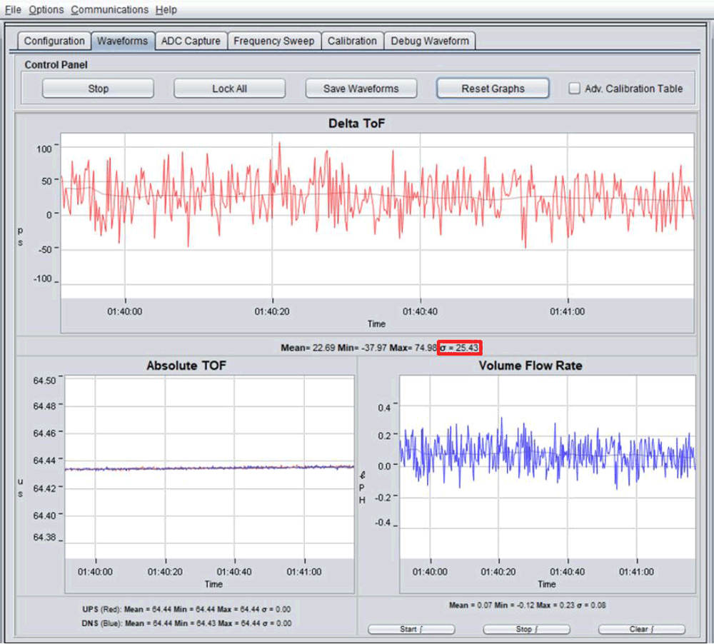
One of the factors that can have a significant impact on the standard deviation is the number of transmit pulses used.
Although increasing the number of transmit pulses can reduce the standard deviation and the number of measurements required to get an accurate reading, it can increase the current consumption. Although increasing the measurement rate can more give a more accurate average, the amount of current consumed will scale based on these additional measurements. Assuming active current consumption of 3uA and sleep current of 1uA at 1 measurement per second, at 4 measurements per second the current consumption would be 12uA of active current with 1uA of sleep current. Similarly, the current consumption can be reduced by reducing the measurement rate when the delta Time of Flight indicates zero flow. Although 2MHz transducers can enable smaller form factor designs, they haven't been observed to provide improvements in standard deviation. We’ll revisit this topic in the context of repeatability and parameter optimization or selection.

Zero Flow Drift Testing

Zero flow drift testing determines the variation in the delta Time of Flight that occurs over the range of operating temperatures at zero flow. This test is important in determining the minimal detectable flow of a water flow meter and accuracy in low flow over its operating temperature range.

Zero flow drift tests are typically conducted in an oven with a temperature profile ranging from 5°C to 85°C over a period of 4 to 24 hours, depending on the robustness of the test. If the climatic chamber is large enough, multiple platforms and pipes can be tested simultaneously.

These tests are conducted with both the meter and electronics in the oven as well as with just the meter in the oven to ensure the electronics do not contribute to the drift. The more important test is when the meter alone is inside the oven.

ZFD Setup

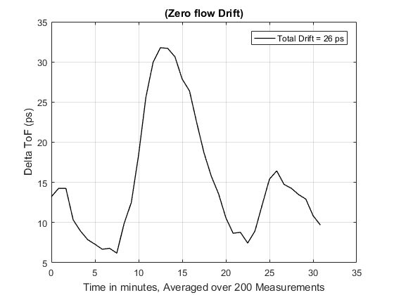
Make sure the pipe with transducers is filled with water ensuring the transducers are fully immersed in water, the same way the testing was conducted for standard deviation. The pipe should be placed in the oven and waveform data should be collected while the oven cycles from +5C to +85C in a series of steps over several hours. Depending on the market requriements or product specifications, the temperature range can be relaxed to +5C to +55C.

ZFD is calculated by obtaining the range of the differential ToF averaged over 200 samples. The MSP430 Ultrasonic Design Center GUI can be used to capture the differential ToF, while tools like MATLAB or Excel can be used to calculate the average over 200 samples and the total drift. The zero flow drift in the delta Time of Flight is depicted in the figure below.

Zero Flow drift of dToF over Temperature with meter in oven:

ZFD Analysis

Because the zero flow drift can improve with impedance matched transducers, it’s important to test a representative set of transducer pairs randomly selected from a production lot (at least 10). Variations in zero flow drift across transducer pairs should be statistically understood when determining the minimum detectable flow of meters in mass production.

Variable Flow Rate Testing

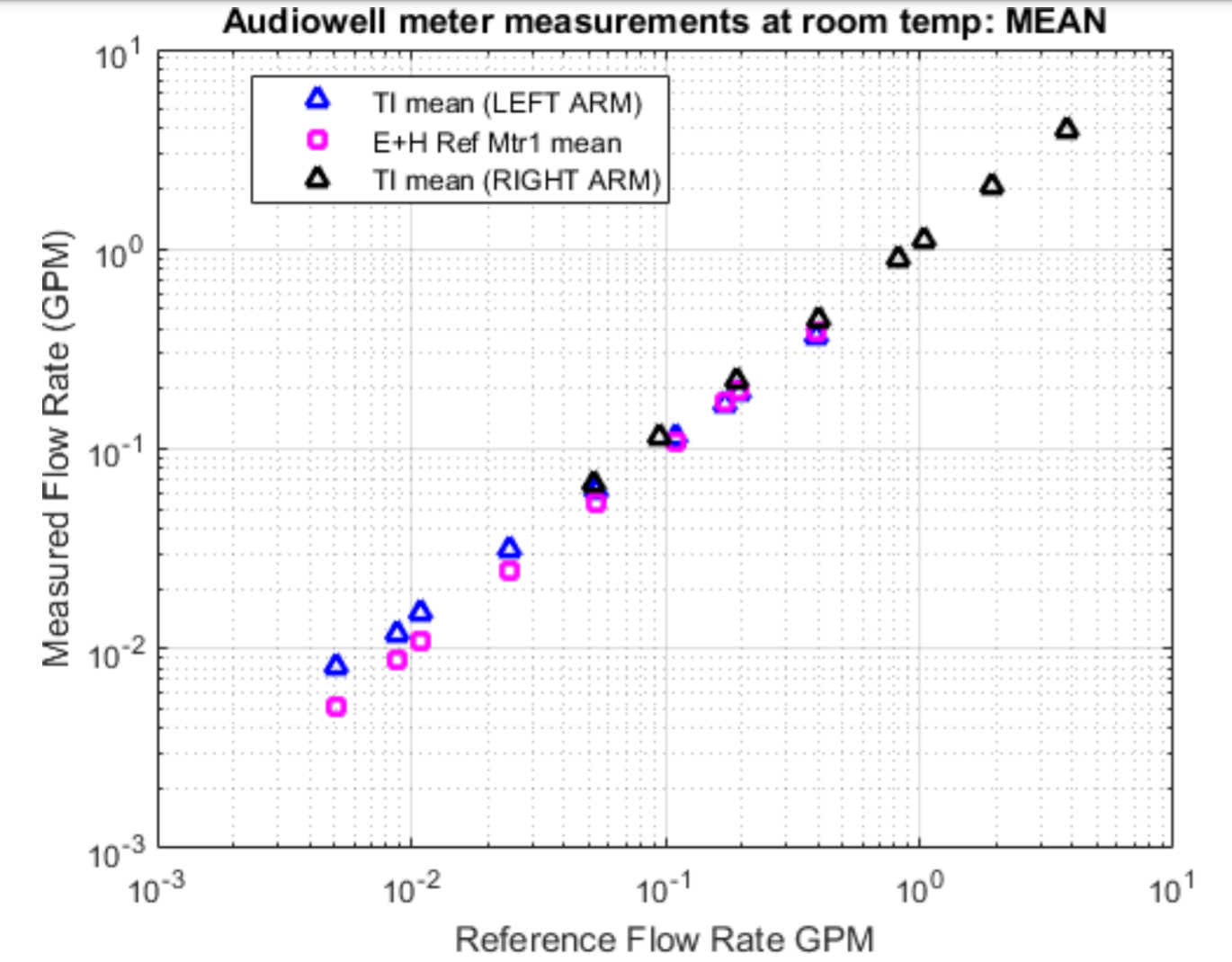
Flow testing is typically conducted with a reference meter and a temperature controlled water circulation system. The figure below shows a typical flow test setup. This setup includes a large water tank, two reference meters, and a Device Under Test (DUT). Flow is recorded at various flow rates by one of the two reference meters and the DUT. The temperature of the water is varied by addition of ice or hot water to the tank with a thermocouple recording the water temperature.

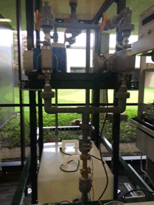
Measured vs Reference Flow Rate:

Flows are typically captured over several minutes and averaged to compare accuracies between a reference meter and the DUT. The figure below shows the comparative flow tests results for a meter at various flows rates across the flow rate range that needs to be supported by the water flow meter.

Uncalibrated Error Plot:

The measured flow rate vs. reference meter flow rate can be used to generate the flow rate accuracy plot or % error plot along the flow rate range that is supported by the meter.

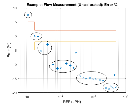
This % error plot clearly shows that with the measured VFR, the error % can vary significantly across the supported flow rate range. This can be reduced by a redesign of the mechanical meter. This is outside the scope of this academy. Here we provide a mechanism to calibrate the uncalibrated flow rate to reduce the error % such that it is within the requirement.

Repeatability Testing

Repeatability testing ensures that there aren't any transient noise issues which might be polluting measurement results. Repeated measurements are expected to give measurement results where the accuracy errors of a given pipe is within 1/3 of the targeted accuracy at a given flow rate and operating temperature. For example, if the accuracy error requirements are 2% at that flow rate and temperature, the variations across repeatability testing should be within 0.67% of the average of the measurement errors. This can be done at multiple flow rates, 1 low, 1 medium, and a high flow rates at room temperature.

Repeatability Test Setup

The same test setup used for variable flow rate testing can be used for repeatability testing of two pipes at the same time. These pipes will need to be in series. Repeatability tests should also be conducted with a calibrated flow test setup to enable comparative debug of issues which might be introduced by the test setup. It's important to note that the transducers should not be removed/replaced between repeatability tests as small changes in the physical distance between transducers can affect repeatability results.

Cycle Slips in Waveform Data:

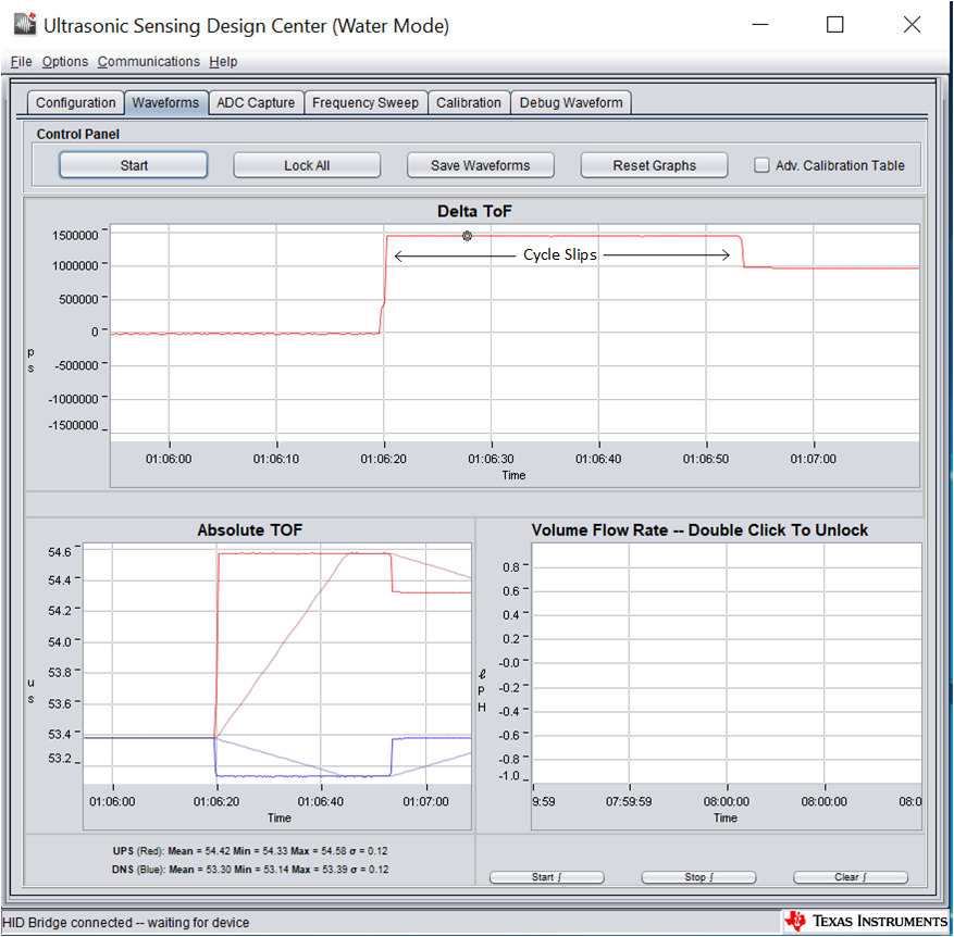
Cycle slips might also occur at higher flow rates due to changes in the ADC capture which cause the absolute time of flight measurement to shift by more than half a cycle. Modifying the tube design to reduce the velocity of the flow in the tube can resolve these problems.

When capturing repeatability data, independent trials should be repeated at least 3 times at target flow rates. The variations in reported measurement results should then be determined to identify potential issues with the tube design or the test environment.

Repeat Measurements:

The standard deviation of results can be improved by capturing more samples if the noise is Gaussian. The accuracy of the measurements should increase based on the square root of the number of samples taken so in order to cut the standard deviation in half, four times as many samples should be used to calculate the mean. In the event that the noise isn’t Gaussian, the noise source must be identified and controlled.

Repeatability testing should also be conducted at representative low, medium and high flow rates at operating temperature extremes (5C and 85C).

Enough experiments should be conducted to determine the statistical probablility that meters will meet specification limits in mass production. This is typically calculated with a Cpk metric. The formula for the calculation of Cpk is Cpk = min(USL - μ, μ - LSL) / (3σ) where USL and LSL are the upper and lower specification limits, respectively. A process with a Cpk of 2.0 is considered excellent, while one with a Cpk of 1.33 is considered adequate.

Calibration of Flow Rate

Calibration of the measured flow rate is done to ensure the error % is within the specification.

Calibrated Error Plot:

Below is the same error % plot along flow rate range shown previously after calibration.

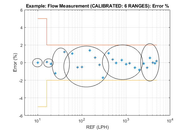
This % error plot clearly shows that with the measured VFR, the error % can vary significantly across the supported flow rate range. This can be reduced by a redesign of the mechanical meter. This is outside the scope of this academy. Here we provide a mechanism to calibrate the uncalibrated flow rate to reduce the error % such that it is within the requirement.

Calibration across Temperature and Flow Rate

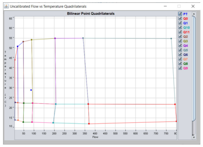
For some pipe designs, and meter requirements that need to support a wide flow rate range and temperature range, the calibration of the measured flow rate also needs to be done as a function of temperature to ensure the error % is within the specification. In these cases, a 2-dimensional calibration is applied along the flow rate axis as well as the temperature axis.

An external temperature sensor can be used to obtain the temperature of water or a temperature estimate can be made using the absolute time of flight measurement.

A typiacl calibration points can be seen in the figure below. The x-axis below is the flow rate and the y-axis is temperature. Each of the quadrilateral points (flow rate, temperature) can be specified through the USS Design Center calibration panel.

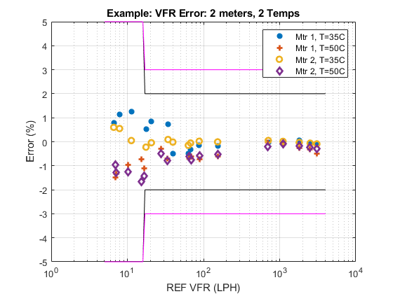
After calibration, the error % of the flow rate can be within the acuracy requirements. This needs to be tested across multiple meters and different temperatures. Below is the error % plot of the calibrated errors for 2 meters and across 2 temperatures.