RTLS Toolbox
The RTLS (Real Time Localization System) Toolbox, is a collection of RTLS techniques that can be implemented on TI’s standard Bluetooth low energy radios in the CC26xx series. These techniques provide raw data that can be used for localization, tracking, and securely range bounding other Bluetooth Low Energy nodes.
The inherent flexibility of the CC2640R2F RF Core is what enables this significant extension of functionality. The main advantages usin CC2640R2F are that customers can start adding RTLS features and security with little or no extra cost, very little to no extra energy consumption and no increase in peak power.
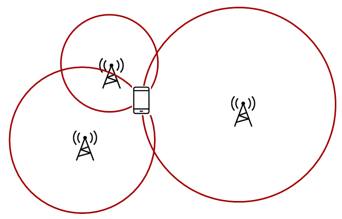
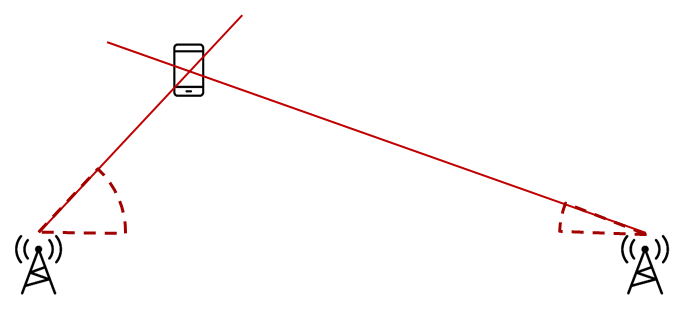
There are two fundamentally different approaches for localization:
| Trilateration | Triangulation |
|
|
Trilateration is where you know the distance between a reference node and a target node. This means that the possible locations seen by one locator constitute a circle, so typically three locators are needed to find a single common intersect point. (Assuming a 2D scenario) Time of Flight gives you the distance from the receiver to the transmitter. |
Triangulation is where you know the direction from a reference node to a target node. This means that the possible locations seen by one locator constitute a straight line, so two nodes will be enough to determine a single intersect point. (Assuming a 2D scenario) Angle of Arrival gives you the angle from the receiver to the transmitter. |
Note
Existing examples with no external control interface are discontinued. All RTLS examples now have an external control interface.
General RTLS Software Architecture
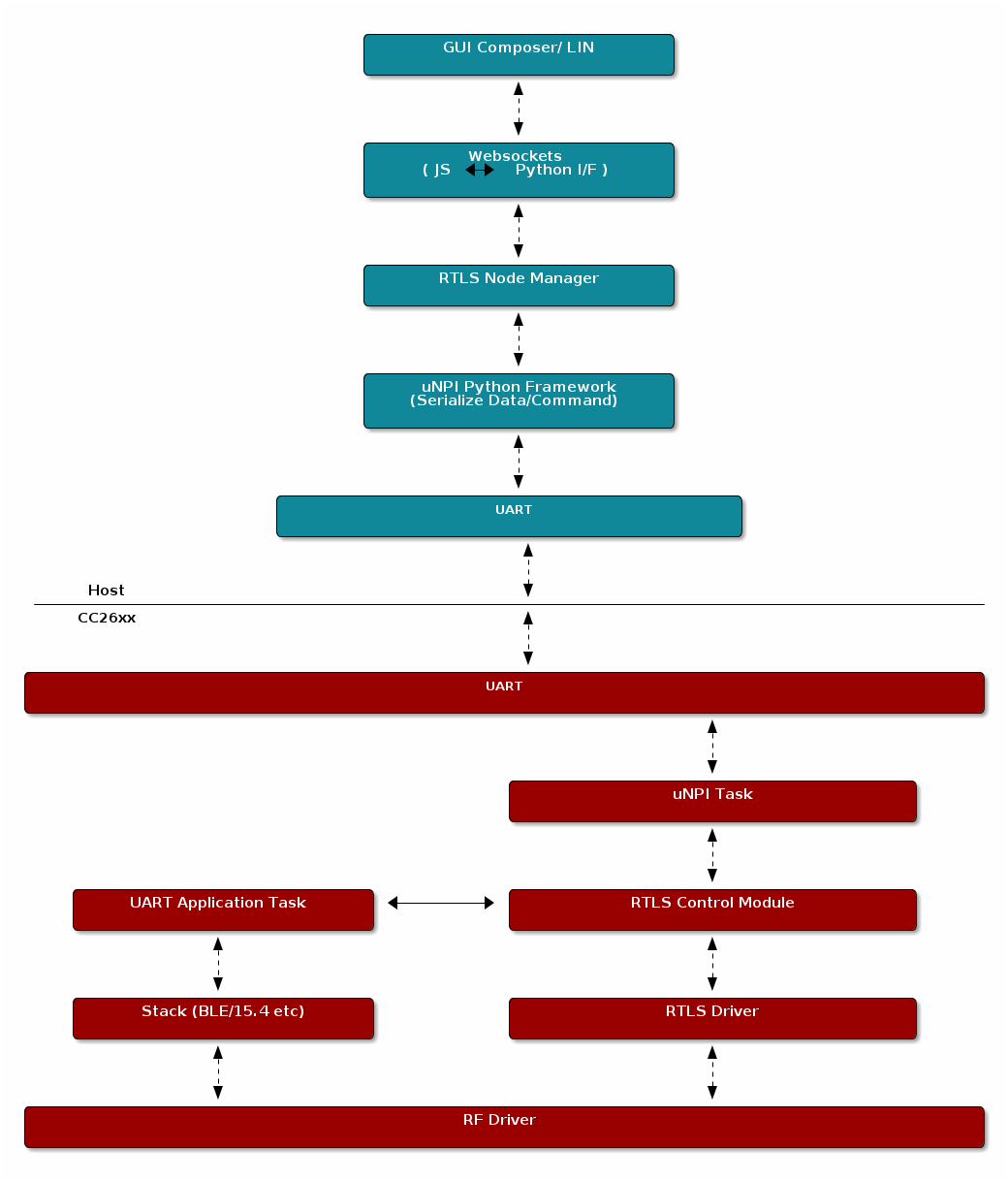
The diagram below shows the RTLS software architecture.
With multiple nodes that collect localization data, it is important to have an architecture that supports control of these nodes. It must be possible to configure and trigger localization and it must be possible to retrieve localization data. We achieve this by reuse of our Network Processor Interface (NPI). It is basically a means to support Remote Procedure Calls (RPC) over a serial interface. Note that the architecture is such that it is possible to replace NPI with your own preferred serial protocol.
In our example we use UART as the serial transport layer. This is because it is readily available on host PC as UART over USB, and our LaunchPads include a UART to USB bridge. Along with the embedded examples we provide PC software to act as host, to control, retrieve and present localization data. This also allows much quicker customer performance characterization, as well as configuration of important parameters, not to mention the ability to develop and test higher level post-processing algorithms.
RTLS Node Manager
The RTLS Node Manager provides the following functionality:
- A bridge between GUI composer and CC2640R2F
- Holds the state of each device and takes care of configuration
- Enables the simplicity of RTLS Control Module and GUI Composer
- Minimizes amount of the transactions between GUI Composer and the rest of the system
Due to the above functionality, the Node Manager can operate on user’s CPU and help with slow bus(LIN/CAN).
RTLS Control Module
The RTLS Control Module is an on-chip module which runs as a RTOS Task and it provides the following functionality:
- Parsing commands coming from Node Manager
- RTLS Driver configuration and operation
- RF and NPI message queue
RTLS Driver
The purpose of RTLS Driver is to handle the Direct Call implementation of the RTLS module.
For more detail please take a look at ToF Driver section and AoA Driver section.
Angle of Arrival
Angle-of-Arrival (AoA) is a technique for finding the direction that an incoming Bluetooth packet is coming from, creating a basis for triangulation.
An array of antennas with well-defined properties is used, and the receiver will switch quickly between the individual antennas while measuring the phase shift resulting from the small differences in path length to the different antenna.
These path length differences will depend on the direction of the incoming RF waves relative to the antennas in the array. In order to facilitate the phase measurement, the packet must contain a section of continuous tone (CT) where there are no phase shifts caused by modulation.
Packet Format
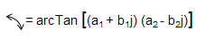
In order to get a good estimate of ϕ (phase), all other intentional phase shifts in the signal should be removed. AoA packets (based on the BLE PHY) achieve this by adding a section of consecutive 1’s at the end of connection packet, effectively transmitting a single tone at the carrier frequency + 250kHz.
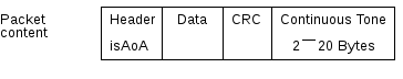
This gives the receiver time to synchronize the demodulator first, and then store I and Q samples from the single tone 250kHz section at the end into a buffer and the buffer can then be post-processed by an AoA application
Note
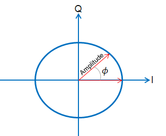
The I/Q Data Sample is the coordinates of your signal as seen down the time axis. In fact, I/Q data is merely a translation of amplitude and phase data from a polar coordinate system to a Cartesian (X,Y) coordinate system and using trigonometry, you can convert the polar coordinate sine wave information into Cartesian I/Q sine wave data.
Integration
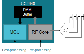
Using a special RF Core patch in receive mode, the I and Q samples from the transmitted carrier frequency + 250kHz tone can be captured, pre-processed, and buffered by the RF Core without any load on the main MCU.
Due to the pre-processing, the application can determine the phase shift without having to remove DC offset or IF first, significantly simplifying the estimation process and leaving the application MCU free to do more on top.
The I/Q samples can be captured at a rate of up to 4 MHz and a resolution of 16 bits (32 bits per I/Q data pair) -> 128 bits/μs -> 1kB holds 64 μs and the buffer size can be up to 2kB (128us of 4MS/s data)
The RF Core can provide event which can be mapped to DMA to trigger the start of GPTimer. The GPTimer is configured as 4us count down mode, once it reaches 4us, then it will generate another DMA transaction to toggle antenna switches.
In slave device, the RF Core patch ensures that the tone is inserted at the end of the connection event packet without being distorted by the whitening filter.
In passive device, the RF Core patch analyzes the packet and starts capturing samples at the right time while synchronizing antenna switching. The samples are left in the RF Core RAM for analysis by the main MCU
AoA Driver
The AoA driver is responsible for antenna switching and data extraction.
Note
As stated in Integration, in this release only rtls_passive device can capture I/Q sample and triggers the radio event for application to do antenna toggling.
Data Collection Flow
Most the code snippet in this section is included in AoA.c.
The radio configuration is now in urfi.c.
When radio core detects AoA tone info in the received packet,
it can trigger an radio event called RFC_IN_EV4 and we can route
the event to DMA channel 14 as a start trigger for antenna switching.
GPTimer 0A is configure as periodic down with 4us timeout and the timeout(timer match) event is routed to DMACH9 to trigger antenna toggling.
When there is AoA packet received (AOA.c), DMA will transfer patterns to toggle the antennas on the BOOSTXL-AoA board.
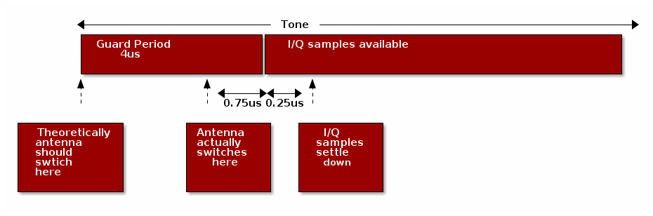
RF core triggers an event 3.25us into the tone.
Therefore to achieve 4us guard time, the AOA_SIGNAL_DELAY_TIME has to be set
to 0.75us, which equals tick number 0.75*48 = 36. The radio core does not collect I/Q
samples in the guard time.
The number for AOA_SIGNAL_DELAY_TIME was found in lab measurement and it’s not recommended to change it.
The method for finding AOA_SIGNAL_DELAY_TIME will be explained in GPTimer Delay Tuning
User can decide how long they want to wait till the antennas
start toggling after the end of the guard time by changing AOA_ANT_SWITCH_START_TIME.
In our example application we set it to 8us (AOA_ANT_SWITCH_START_TIME = 8*48 = 384).
After antenna toggling, you can get the pointer to the IQ samples in radio RAM by the following function.
Then the data get passed into the AOA_getPairAngles() to get the estimated angle between receiver and sender.
GPTimer Delay Tuning
In order to find the signal delay between when the radio core detects AoA packet until GPTimer starts,
we first extracted the I/Q data while setting AOA_SIGNAL_DELAY_TIME = 0 and AOA_ANT_SWITCH_START_TIME = 0.
We observed that the I/Q samples settle down about 0.25us into the sampling time. RF core triggers an event immediately when the tone starts. Firstly it takes ~1us from RFC_IN_EV4 to GPIO’s toggles (600ns for RFC_IN_EV4 -> DMA9, 400ns for DMA9 -> GPIO). Then it takes ~2.25us from the antennas switch until we can see this in the IQ data (delay through RF/IF chain, IF ADC, IQ re-sampler and RAM write).
We already know that the our antenna settling time is 1us, so if we want antenna switching to start at IQ sample[0], AOA_SIGNAL_DELAY_TIME need to be 0.75us (0.75*48).
Antenna Switching
Control pattern is placed in ant_array1_config_boostxl_rev1v1.c and ant_array2_config_boostxl_rev1v1.c: We will focus on code for antenna array 1. The same theory applies for antenna array 2.
The ‘AOA_PIN()’ is just a bitwise operation. If you want to use your own design(different IOs), you will need to change the parameter passed on to AOA_PIN function.
On top of the change made in antenna file, you also need to modify the highlighted part of the code used in the AOA.c.
The initial pattern suggested that in our example second antenna under antenna array group 1 is used to receive the incoming packets at the beginning and the end.
After that, once AoA packet is detected, we will start toggling IOs to choose different antenna in order to gather the phase difference between each antenna. Here we use GPIO:DOUTTGL31_0 register to enable the toggling function. For more information, please see Driverlib Documentation CC2640R2F -> CPU domain register descriptions -> GPIO:DOUTTGL31_0
The first antenna used is second antenna which is controlled by IOID_29 and then we want to change to a different antenna(assuming antenna 1 IOID_28). This means that we need to toggle both IOID_29 and IOID_28. Then we need to set both bit[29] and bit[28] to 1 in register GPIO:DOUTTGL31_0 in order to toggle.
In our software solution, the following function is taking care of toggling pattern generation. It takes the previous selected IOID_x and XOR with the current selected IOID_x.
Therefore all you need is to design the pattern and then call the following two functions to initialize the patterns
(assuming you have two arrays).
These two functions are called in AOA.c void AOA_init(AoA_Results_t *aoaResults).
Convert I/Q Data to Angle Difference
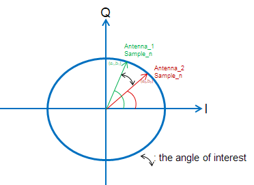
When the radio frequency wave incident on to an antenna array(assuming there are only 2 antennas on the board) and arrives at different antennas at different time, there will be phase difference between the antennas. So we extract the phase difference between ant1_sample[8 to 15] and ant2_sample[8 to 15]. The switch among antennas will cause measurement error, therefore we discard I/Q samples from 0 to 7 when calculating angles.
When using a custom HW with different antenna switch than what we have on BOOSTXL-AoA board, you might be able to use more I/Q samples if antenna switch settling time is shorter than 1us. The method for determining how many I/Q samples can be used is explained in Valid I/Q Samples For Angle Calculation
The I/Q data can be presented into a X-Y domain with real number I and imaginary number Q (90 degree difference). As mentioned before, for each period of 250 kHz signal, we sample 16 I and Q data. If there is no difference, that means that the I/Q data is the same, therefore the phase between ant_1 sample1 will be the same to ant_2 sample1.
Here is the code putting I/Q data into 2 dimensions and then we passed the I/Q pairs into function
AOA_AngleComplexProductComp() to get final angle.
The reason for having a 32 offset for the sample array is that because the we use
8us as guard time(controlled by AOA_ANT_SWITCH_START_TIME). 8us guard time with 4MHz sampling rate
gives us 32 samples, therefore we take the I/Q samples after the guard time.
For users that want to have different guard time, the offset should be calculated as ‘guard time (in us) x sampling rate(in MHz)’.
Something to highlight is that in reality the 250kHz might not be perfect (for example, could be 255kHz or 245kHZ), therefore, there is slightly phase difference between ant_1 sample_n and ant_1 sample_(n + 16*1). Therefore run time compensation is also applied:
Because of the none perfect 250kHz tone, the phase difference is aggregated. Let’s say that every period will have 45 degree of delay. Then when comparing ant_1 sample_n and ant_1 sample_(n+16*1), the aggregated phase difference is 90 degree. But the real phase difference between every period is only 45. Therefore the calculated phase difference must be divided by the number of antennas used, in our case 2.
Valid I/Q Samples For Angle Calculation
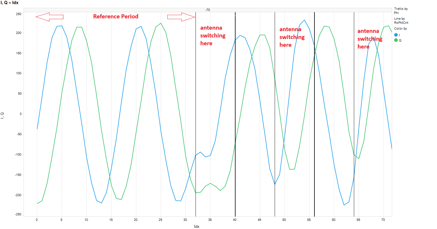
In order to determine what I/Q samples to use. The easiest way to tell is to plot all the I/Q samples.
The picture below shows the I/Q samples which were collected using our rtls_passive example together with rtls_master and rtls_slave examples.
Table 20. Axis description¶ Axis Description X top Angle between a rtls_slave device and rtls_passive. X bottom Index number of I/Q data. Y I/Q values.
The first 32(index 0~31) samples are taken in reference period which there is no antenna switching. Therefore the I/Q plot looks like sinusoid wave.
After that at index 32, you can see when switching happened there comes discontinuity of I/Q samples.
Note
It’s easier to see the phase discontinuity when there is indeed phase difference. Therefore, before collecting I/Q data, make sure the angle between rtls_passive and rtls_slave is not 0 degree.
Angle Compensation
Under AoA_getPairAngles(), we will acquired the angle based on I and Q data. After that, angle compensation is added. Please see the code below. This is because angle estimation is affected by antenna pairs and frequency. The values p->gain, p->offset, channelOffset_A1 and channelOffset_A2 are based on lab measurements. Different antenna board design and frequency will give you different p->gain, p->offset, channelOffset_A1 and channelOffset_A2.
The following code can be found in AOA.c AoA_getPairAngles(), this is antenna pairs compensation.
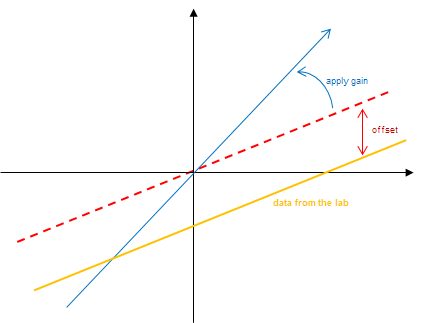
As you can see from the image above, the offset is applied to make sure the data received at 0 degree will derive 0 degree after the calculation and then the slope is changed to make it fit better with all the rest of the angles.
The compensation values for antenna array 1 can be found in
ant_array1_config_boostxl_rev1v1.c AoA_AntennaPair pair_A1[]
Followed by antenna pair compensation, we added frequency compensation.
For antenna array 1, the values used for frequency compensation can be found in
ant_array1_config_boostxl_rev1v1.c int8_t channelOffset_A1[40].
AoA Functions Overview
The functions covered under this section are all in AOA.c.
AOA_init:
For
rtls_passivedevice, this function takes care the following HW initialization.- Initialize GPIOs
- Set up I/O toggling patterns
- Route needed signal to DMA channels
- Set up GPTimer
For
rtls_slavedevice,AOA_initwill get the size of the RF override table.AOA_cteCapEnable:
For
rtls_passivedevice, it extracts the following 3 parameters which are input from users through NPI and then are stored in the RF RAM:- cteScanOvs: This is the I/Q sampling rate for the AoA tone. Table 21.
shows available values for this parameter. Out of box example is made with
cteScanOvs = 4. - cteTime: The length of the continuous tone. The allowed range is from 2~20 in 8us units.
The out of box is made with
cteTime = 20. This parameter in passive is used to calculate the number of available I/Q samples. - cteOffset: This gives the number of microseconds from the beginning of the tone
to the sampling starts The allowed range is from 0~63. Out of box example is
made with
cteOffset = 4, which means the radio core will wait for 4us at the beginning of the tone till it starts sampling. If this parameter is set larger than the actual tone duration, thecteOffset = 4will be used.
For
rtls_slave, this function sets up the slave to send out continuous tone withcteTime*8usat the end of every connection packet by adding 1 extra override right before the end of the last override(0xFFFFFFFF).Table 21. cteScanOvs setting¶ Value Description 0 No special processing of AoA packet. 1 Process packets with AoA present in the header and sample the tone at 1 MHz.(not recommended, because this provides very little I/Q samples) 2 Process packets with AoA present in the header and sample the tone at 2 MHz. 3 Process packets with AoA present in the header and sample the tone at 3 MHz. 4 Process packets with AoA present in the header and sample the tone at 4 MHz. 15 Process packets with AoA present in the header but do not sample the the tone. - cteScanOvs: This is the I/Q sampling rate for the AoA tone. Table 21.
shows available values for this parameter. Out of box example is made with
AOA_calcNumOfCteSamples
This function is only needed for
rtls_passivedevice to decide how big the array needs to be for I/Q samples and how many samples are avaiable per antenna. For example, if we take cteScanOvs = 4, cteTime = 20 and cteOffset = 4, then we should get ( cteTime*8 - cteOffset ) * cteScanOvs = 624 I/Q pairs. However, the radio RAM can only store upto 512 I/Q pairs. When this situation happens, the radio core will stop I/Q sampling once it fills up the radio RAM for I/Q storage area.AOA_cteCapDisable
For
rtls_passivedevice, this function will disable I/Q sampling and ignore AoA present in the header.For
rtls_slavedevice, this function will disable slave device to send out continuous tone.
Time of Flight
ToF is a technique used for secure range bounding by measuring the round trip delay of an RF packet exchange.
This is implemented in a Master-Slave-Passive configuration, where the Master sends a challenge and the Slave returns a response after a fixed turn-around time. The Master can then calculate the round trip delay by measuring the time difference between transmission of the challenge and reception of the response, subtracting the (known) fixed turn-around time. Passive will not participate in the exchange over the air, but will also measure the observed Time of Flight.
Due to the low-speed nature of a Bluetooth radio when evaluated in a speed-of- light-context, each individual measurement provides only a very coarse result. But by performing many measurements, typically several hundred within a few milliseconds, an average result with much better accuracy can be achieved.
Theory of Operation
Few things are faster than the speed of light, and that speed is known and constant at c. Electromagnetic waves propagate at the speed of light, and thus an RF packet propagates at the speed of light.
Since the speed is constant, this means that the time it takes for a wave to propagate is directly proportional to the distance. To find the distance to an object, we can record the timestamp when we transmit something and compare this to the timestamp when the reflection is received, divide by two and multiply by c. This is the operating principle of for example RADAR as well.
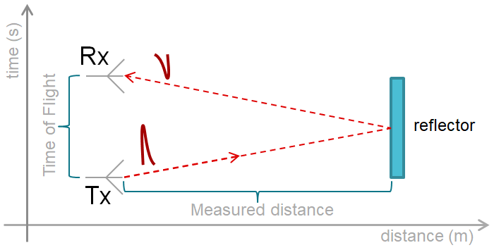
Figure 76. Reflected EM wave. If time between transmit and receive is t, then distance d is simply ct/2.
As opposed to RADAR, the reflector in TI ToF is considered active as it
does not reflect the outgoing signal meaningfully but instead must actively
send out the “reflection”.
There are at least two main challenges when doing this form of measurement:
- The time the reflector uses between receipt of the
PINGand transmission of thePONGwill affect the measured distance. - Light uses 3.3ns to travel one meter, which means that the tick speed of a clock measuring the time of flight must apparently be at least 303 MHz to get 1m spatial resolution.
The first challenge is overcome in the TI ToF solution by implementing a deterministic turn-around time in the slave/reflector device.
The second challenge is overcome by taking a statistical approach to measuring the distance. The frequency of the radio timer used to measure Time of Flight is 8 MHz, which means that the temporal resolution is 125 ns. The accuracy of the final measurement can be improved by oversampling the individual packet measurements. This is because there is jitter in the sample, and this jitter has a normal distribution. In order to achieve higher accuracy, the time of flight will be measured over many PING/PONG exchanges across multiple devices. Resolution is discussed further in the Resolution section and accuracy is discussed in the Accuracy section.
Terminology
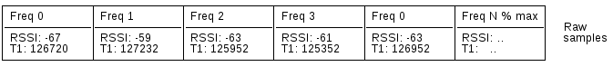
PING: A packet sent to initiate a ToF measurementPONG: The response packet to a PINGRun/burst: A series of PING/PONG exchanges that are used to measure distanceTick: A single period of the RF core clock that is used to measure ToFSample: The measured RSSI, tick, and channel infomation for a single PING/PONG exchange
To recap, a ToF burst is a collection of PING/PONG exchanges. Each PING/PONG exchange results in a ToF sample which is a collection of RSSI, timestamp (in number of ticks), and frequency information. A burst can contain a configurable amount of PING/PONG exchanges and may operate on a configurable list of frequencies. At the end of a burst, all tick information can be averaged to form an estimate of distance. Information from multiple bursts across multiple devices can be combined to form a distance measurement within a given confidence interval.
Packet format
The modulation format is 2Mbps at 500kHz deviation using a piecewise linear shaper for the transitions. Packet content is based on a standard BLE packet with some modifications to meet the ToF usecase.
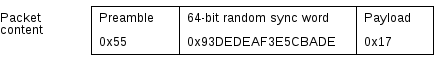
The packets contain a random pre-shared sync word that is unique for each frame sent over the air, and that either side will be listening for in their RX cycle.
The syncword is how the RF circuitry detects that the packet is intended for the device, and also how the timestamps are generated for the measurements.
Note
Security in ToF is dependent on a good syncword generation algorithm. Syncwords should not be easily guessable by an attacker and should not be repeated. Instead they should be generated in a manner such that the trusted ToF nodes are able to determine the next syncword, but an attacker cannot. See Security
ToF Roles
There are three roles supported by the ToF solution.
Master: Initiates ToF sequence by sending PINGSlave: Listens for PING, responds with PONGPassive: Listens for both PING and PONG
Master and passive will measure the Time of Flight using a timer in the RF core. While the passive role is not strictly required to run ToF, it will increase the robustness of the measurement by adding additional samples into the measurement.
Since ToF is a statistical measurement, with more samples comes a higher degree of confidence in a given measurement. Passive nodes also add spatial diversity and can reduce the effects of reflections and multi-path fading in a ToF measurement. There is no limit to the number of passive nodes that can be added, but there must be at least one master and one slave.
The distance between ‘’Passive’’ and ‘’Master’’ must be known, so that this distance can be calibrated out.
ToF Protocol
The Master and Slave devices will listen and transmit on a range of
frequencies provided by the application.
Meanwhile, the Passive device will listen to all the packets transmitted
between Master and Slave after they have achieved sync.
The Slave is initially in receive mode on the first frequency and is
listening for the first syncword SW0, this is the PING.
If the slave receives a matching packet in the initial listening period it
will send a PONG and will start following a time-slotted scheme where
it changes frequency and syncwords.
The master will send out a packet containing the first syncword(SW0) and some application defined payload. Immediately after this it will go into receive mode and wait for a slave to reply transmitting the second syncword(SW1) in the array.
Similarly, if the master receives a matching ACK/PONG packet in response
to the initial PING, it will follow the same time-slotted and frequency-
hopping scheme.
The passive will begin in RX mode, waiting for SW2
Once the Passive receives SW2, it will start following
the time-slotted and frequency hopping scheme.
Passive starts the radio timer when it receives SW2n, and then stops the
timer once Passive receives SW2n+1.
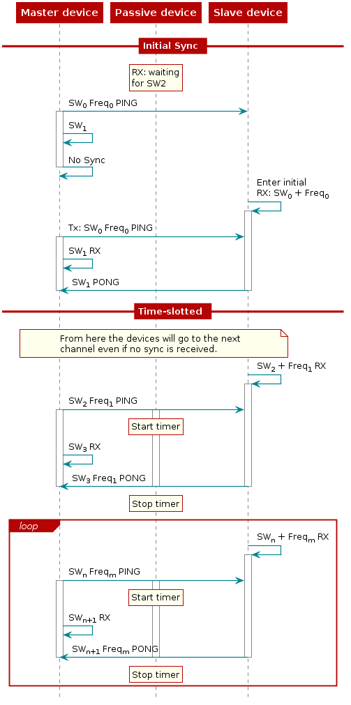
Figure 77. ToF measurement-burst sequence
If we consider the timing of the packets, we can try to illustrate the time of flight as the distance between the two first vertical lines below.
You can see that the internal clocks of the two devices are not syncronized, illustrated by the top line for each device, and you can see the three phases of a ToF measurement:
- Master sends PING, Slave receives
- Devices switch RF roles, TX to RX and RX to TX
- Response PONG is sent
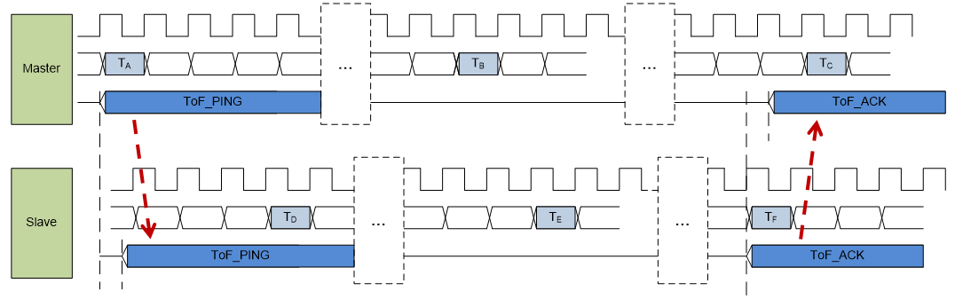
Figure 78. ToF Timing diagram. See legend below.
Resolution
Distance in ToF is measured in ticks of the radio timer, which runs at 8MHz. These tick values must be converted to meters in order to estimate the distance to the slave. The distance equation is used to perform the conversion. This section seeks to show step-by-step derivation of the tick to meter conversion constant.

Since ToF packets are EM waves, their propagration rate is fixed at c,
the time it takes for light to travel one meter. The result must be
divided by 2 since the time accounts for the round trip travel time of the
packet which is 2x the actual distance.
In order to convert tick values into time, they must be divided by the frequency of the RF core timer. Substituting this into the distance equation above gives the scaling factor used to convert ticks into meters.
![\begin{align*}
\begin{split}
\text{distance} &= \frac{1}{2}\times\text{t}\times\text{c}\\[16pt]
&= \frac{1}{2}\times\frac{\text{tick}}{8\si{\mega\hertz}}\times\text{c}\\[16pt]
&= \frac{\text{tick}}{2\times8\times10^{6}\text{s}^{-1}} \times 3\times10^{8}\si{\meter/\second}\\[16pt]
&= 18.75\si{\meter}\times\text{tick}
\end{split}
\end{align*}](../_images/math/1abcea4791d74fc4b5ceaac4f74f7c9f37b581b1.svg)
A ToF packet will travel 18.75 meters per tick. In software, this constant
is referred to by TICK_TO_METER. To convert a tick value to meters simply
multiply by TICK_TO_METER.
Accuracy
Inside the RF core of the CC2640R2F there is a component called the correlator. The correlator is responsible for measuring the correlation value between two syncwords. When the RF core is running a ToF command, the correlator is responsible for starting and stopping the timer that measures ToF ticks.
The various devices in the ToF toplogy do not have a method for synchronizing their clock, and therefore there is some inherent phase noise in the clocks in comparison to each other. This means that over multiple ToF samples the time at which the correlator reports sync will drift slightly. This is illustrated by the gif below.
It is the correlator that is responsible for starting and stopping the timer that reports ToF ticks. Phase noise causes spreading in the “sync found” point in time and thus spreading occurs in the ToF results. Over many samples in a ToF run, the ticks will be spread around the true correlation point in a normal distribution.
Plotting ToF results as a histogram for a given distance and number of samples yields results similar to the figure below.
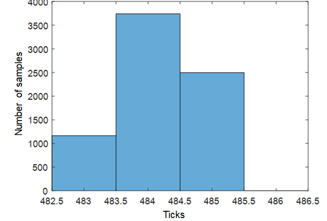
Using a concrete example based on the histogram above, we have the following results:

In the true distance calculation, we must account for calibration.
Calibration will be covered in depth in the Calibrate section.
For now, assume the calibration value is measured in ticks and is 484.

Plugging in the results from the histogram above results in
![\begin{align*}
\begin{split}
\text{$tick_{avg}$} &= \frac{\text{$count_{483}$}\times483}{count_{total}} + \frac{\text{$count_{484}$}\times484}{count_{total}} + \frac{\text{$count_{485}$}\times485}{count_{total}}\\[16pt]
&= 484.1756757
\end{split}
\end{align*}](../_images/math/2726168712dd048ee755b74e2d71a11f71f0b1cf.svg)
Plugging in the tick_avg to the final equation yields the following:

This example demonstrated the concept that ToF becomes more accurate with increased sample number. It also shows how ToF can be used to measure distances of less than 18.75m thanks to the spreading introduced by phase noise.
ToF Driver
The ToF driver is responsible for managing setting up the Time of Flight RF command, and interfacing between the RF driver and the application. Additionally, the ToF driver will use the ToF Security module to generate random seeds. Furthermore, the ToF Security module will use the random seeds for secure syncword generation using the Advanced Encryption Standard Counter Deterministic Random Bit Generator (AESCTRDRBG) algorithm.
From the application, it is relatively simple. You need to:
- Initialize
- Run
- Collect the results
- Calibrate
Initialize
The ToF driver needs a parameter struct with some information filled in. The example has this filled in already, but the most interesting parameters are:
tofRole- Device role: Master/SlavepT1RSSIBuf- Pointer to sample bufferpSyncWords- Pointer to array of syncwordsnumBurstSamples- Number of syncwordsfrequencies- Pointer to array of frequenciesnumFreq- Number of frequenciespfnTofApplicationCB- Callback after run.tofSecurityParams- Security configuration parameters
The sample buffer must be at least numBurstSamples / 2 large. The list of
frequencies and the list of syncwords must be identical on both sides.
Hint
The numBurstSamples actually describes the number of syncwords to be
in the ToF burst. Since it requires two syncwords (PING + PONG) to produce
a single sample, the actual number of samples is numBurstSamples / 2
You must also allocate space for the ToF driver instance, a struct of the type
ToF_Struct.
Once that’s done, you can call
ToF_Handle handle = TOF_open(&tofStruct, &tofParams);
Security
The security of ToF is based on the premise that an attacker is unable to guess the next syncword to be used in the ToF run. This means that syncwords must never be recycled. If an attacker can easily guess the next syncword, the system is susceptible to replay attacks.
Instead, a random seed is distributed to the ToF responder using an encrypted connection. This seed is distributed to ToF passive nodes using a serial connection.
This seed is then fed into the AESCTRDRBG algorithm to generate a new table of syncwords. These syncwords are then used for ToF. In order to optimize the use of the radio while generating a new syncword table, the syncword list is double buffered so that the security module can be generating new syncwords while the RF core is consuming them.
Random seed
The random seed is generated using the True Random Number Generator (TRNG) hardware module and driver. This is distributed to via GATT profile.
AESCTRDRBG
The syncword table is generated using AES-128 block algorithm based on section 10.2.1.2 of NIST SP 800-90Ar1. This will use the Crypto driver in polling mode.
Run
When you call TOF_run(handle, tofEndTime) it will start immediately.
When combined with Bluetooth, you will get the time in Radio Access Timer
(RAT) ticks from the BLE Stack to use as ToF end-time.
Note
tofEndTime is measured in ticks of the Radio Access Timer (RAT) that runs at 4 MHz. It is important to remember that this is different than the RF core timer that runs at 8MHz that is used to measure ToF.
The tofEndTime parameter is valuable when scheduling ToF events in between stack communication such as Bluetooth.
Collect the results
This is done in the callback function given in the initialization parameters:
ToF_BurstStat tofBurstResults[TOF_MAX_NUM_FREQ] = {0};

void myCallback(uint8_t status) {
  TOF_getBurstStat(tofHandle, tofBurstResults);
  // Do something
}
This function takes the interleaved raw samples and averages them per frequency.
The raw samples are stored in a flat list (above), but the statistics function presents them per frequency:
typedef struct
{
    uint16_t freq;          // Frequency
    double   tick;          // Time of Flight in clock ticks, averaged over all valid samples for `freq`
    double   tickVariance;  // Variance of the tick values
    uint32_t numOk;         // Number of packets received OK for `freq`
} ToF_BurstStat;
The tick value can be converted to meters by subtracting the calibrated tick
value at 0 meters and multiplying with 18.75.
Calibrate
The measured Time of Flight will be longer than the actual Time of Flight. The error in measurement is caused by the following quantites:
- Slave turnaround time (switch from RX to TX)
- Intrinsic delay of device when using ToF PHY
These quantities are deterministic and non-zero. They differ slightly between devices based on the characteristics of the silicon. These characteristics will not change through the lifetime of the device, thus calibration must only be performed once per device and can be stored.
The following components make up a ToF measurement on master:

The following components make up a ToF measurement on passive:

Acting in a master role, each ToF measurement contains two delay components that should be calibrated for, the intrinsic delay of each device, and the turnaround time in the slave. Assuming a system of three devices, the master can be rotated to produce the following results, where M_12 denotes the ToF measured where device 1 is master and device 2 is slave. Note that below assumes ToF=0

Solving these equations results in the following:

Solving the above systems of equations gives the intrinsic delay of each device when operating as a master.
The same can be done for passive, keeping in mind that a passive measurement contains the delay from all three devices (master, slave, passive). For example with ToF=0. In the following equations, the following convention is used. P_123 represents as passive ToF measurement where is device 1 is passive, device 2 is master, and device 3 is slave. We will introduce a 4th device while calculating the passive delay, to show how the system scales as passive devices are added.

Rotating the passive role throughout the devices gives the following system of equations, note that here we are assuming that there are 4 passive devices. The method below can be scaled as more devices are added.

Solving this equation results in:

These delays should be measured in a controlled environment at production time in order to characterize the deivce, and should be stored in non volatile memory so that they can be used to adjust all ToF measurements.
Application
The application has to somehow agree with the peer device(s) what frequencies should be used, the order of frequencies, and what the list of syncwords should contain.
In addition, it must call ToF_run(...) at appropriate times to initialize
the initial syncword search and the time slotted measurement burst.
This can also be shown as a (very) simplified sequence diagram:
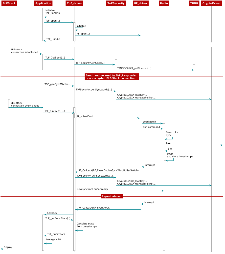
Figure 79. ToF Application Example
Interleaving with Bluetooth
A Bluetooth LE device in a connection is bound to wake up and transmit or
receive at certain times known as Connection Events. The interval between
such events is called a Connection Interval.
The Passive device is integrated with connection monitor functionality,
therefore, it can obtain connection information(rssi, timestamp) and also
listens for ToF packets at the end of each connection event and providing
calculated distance.
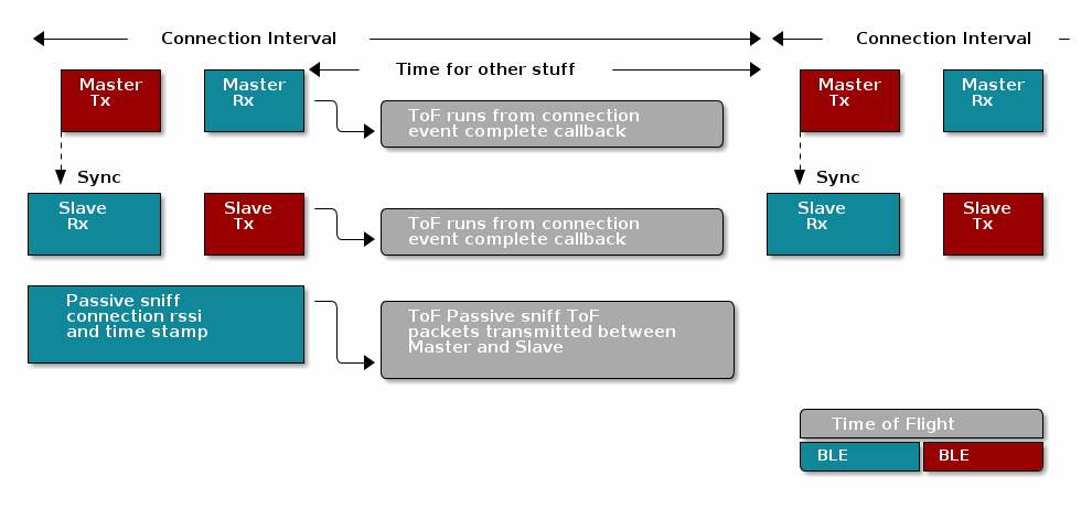
In the time between the end of one connection event and the start of the next scheduled connection event, there is time to schedule other RF commands, such as ToF.
The available time can vary, but a time stamp is provided in the connection event complete callback for when Time of Flight has to be finished using the radio.